第 4 节 / 共 7 节
神经网络基础(二):搭建网络
Day04 笔记:神经网络基础(二)
Day 04 - 神经网络基础2
学习目标
- 动手实现搭建神经网络
- 掌握常用损失函数
- 掌握梯度下降算法
- 了解反向传播算法
- 掌握梯度下降的优化方法
# 导包
import torch
import torch.nn as nn
import torch.optim as optim
import numpy as np
import matplotlib.pyplot as plt
# 设置中文字体
plt.rcParams['font.sans-serif'] = ['SimHei']  # 微软雅黑
plt.rcParams['axes.unicode_minus'] = False            # 解决负号显示问题
# 设置设备
device = torch.device("cuda" if torch.cuda.is_available() else "cpu")
day04_01.搭建神经网络
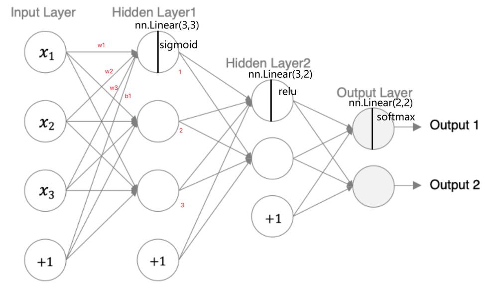
"""
案例:
    演示 搭建神经网络 的流程

要求:
    第1个隐藏层:权重初始化采用标准化的xavier初始化 激活函数使用sigmoid
    第2个隐藏层:权重初始化采用标准化的He初始化 激活函数采用relu
    out输出层 采用softmax做数据归一化,权重初始化采用标准化的xavier初始化

深度学习的一般工作流:
    1.准备数据集
    2.搭建神经网络:
        前向传播方法forward
    3.模型训练:
        构造损失函数 优化器
        前向传播,获取预测值
        计算损失
        梯度清零
        反向传播,计算梯度
        更新参数,梯度下降法
    4.模型测试

搭建神经网络的流程:
    1.定义一个模型类,继承 nn.Module
    2.定义__init__方法,搭建网络层
    3.定义forward方法,实现前向传播

"""

# 导包
import torch
import torch.nn as nn
from torchsummary import summary  # 计算模型参数,查看模型结构, pip install torchsummary
# 设置设备
device = torch.device("cuda" if torch.cuda.is_available() else "cpu")
print(device)
# 1.定义模型类,搭建神经网络
class MyModel(nn.Module):
    # 1.定义__init__方法,搭建网络层
    def __init__(self):
        # 1.初始化父类成员
        super().__init__()
        # 2.搭建网络层
        self.linear1 = nn.Linear(3, 3)
        self.linear2 = nn.Linear(3, 2)
        self.linear3 = nn.Linear(2, 2)
        # 3.参数初始化
        # # 初始化linear1
        # nn.init.xavier_normal_(self.linear1.weight)
        # nn.init.zeros_(self.linear1.bias)
        # # 初始化linear2
        # nn.init.kaiming_normal_(self.linear2.weight)
        # nn.init.zeros_(self.linear2.bias)
        # # 初始化linear3
        # nn.init.xavier_normal_(self.linear3.weight)
        # nn.init.zeros_(self.linear3.bias)
    # 2.定义forward方法,实现前向传播
    def forward(self, x):
        # 1.输出隐藏层1,linear1
        # x = self.linear1(x)
        # x = torch.sigmoid(x)
        # 合在一起
        x = torch.sigmoid(self.linear1(x))
        # 2.输入隐藏层2,linear2
        x = torch.relu(self.linear2(x))
        # 3.输入输出层,linear3
        x = torch.softmax(self.linear3(x), dim=-1)
        # 4.返回输出结果
        return x


# 2.模型训练,演示前向传播,并统计模型参数
def train():
    # 0.设置随机种子,保证结果可复现
    torch.manual_seed(42)
    # 1.创建模型对象
    model = MyModel()
    print(model)
    # # 2.准备数据集,需要是二维张量
    # data = torch.randn(10,3)  # 10个样本,每个样本3个特征
    # print(f"data: {data}")
    # print(f"shape: {data.shape}")
    # print(f"data.requires_grad: {data.requires_grad}")

    # # 3.前向传播,获取预测结果
    # y_pred = model(data)    # 底层自动调用forward方法,实现前向传播,返回预测结果,(10,2)
    # print(f"y_pred: {y_pred}")
    # print(f"shape: {y_pred.shape}")
    # print(f"y_pred.requires_grad: {y_pred.requires_grad}")
    # print("-" * 60)

    # 4.查看模型的参数数量
    print("模型参数情况:")
    model.to(device)
    summary(model, (3,))
    for name, param in model.named_parameters():
        print(f"{name}: {param}")

# 3.测试
if __name__ == '__main__':
    train()
cuda
MyModel(
  (linear1): Linear(in_features=3, out_features=3, bias=True)
  (linear2): Linear(in_features=3, out_features=2, bias=True)
  (linear3): Linear(in_features=2, out_features=2, bias=True)
)
模型参数情况:
----------------------------------------------------------------
        Layer (type)               Output Shape         Param #
================================================================
            Linear-1                    [-1, 3]              12
            Linear-2                    [-1, 2]               8
            Linear-3                    [-1, 2]               6
================================================================
Total params: 26
Trainable params: 26
Non-trainable params: 0
----------------------------------------------------------------
Input size (MB): 0.00
Forward/backward pass size (MB): 0.00
Params size (MB): 0.00
Estimated Total Size (MB): 0.00
----------------------------------------------------------------
linear1.weight: Parameter containing:
tensor([[ 0.4414,  0.4792, -0.1353],
        [ 0.5304, -0.1265,  0.1165],
        [-0.2811,  0.3391,  0.5090]], device='cuda:0', requires_grad=True)
linear1.bias: Parameter containing:
tensor([-0.4236,  0.5018,  0.1081], device='cuda:0', requires_grad=True)
linear2.weight: Parameter containing:
tensor([[ 0.4266,  0.0782,  0.2784],
        [-0.0815,  0.4451,  0.0853]], device='cuda:0', requires_grad=True)
linear2.bias: Parameter containing:
tensor([-0.2695,  0.1472], device='cuda:0', requires_grad=True)
linear3.weight: Parameter containing:
tensor([[-0.3258, -0.0829],
        [-0.2872,  0.4691]], device='cuda:0', requires_grad=True)
linear3.bias: Parameter containing:
tensor([-0.5582, -0.3260], device='cuda:0', requires_grad=True)
4. 损失函数
损失函数概念
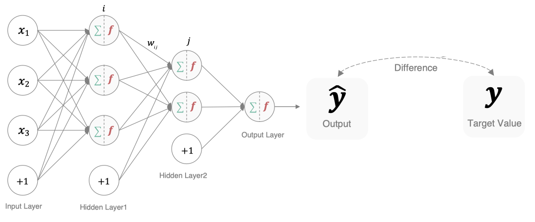
在深度学习中, 损失函数是用来衡量模型参数质量的函数, 衡量的方式是比较网络输出(预测值)和真实输出(真实值)的差异。
我们通过最小化损失函数的值来调整模型参数,使其输出更接近真实值。
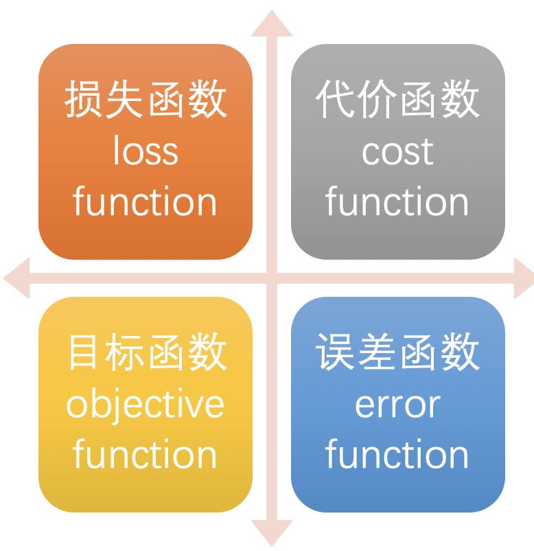
损失函数在不同的文献中名称是不一样的,主要有以下几种命名方式:
损失函数作用:
- 评估性能:反映模型预测结果与目标值的匹配程度。
- 指导优化:通过梯度下降等算法最小化损失函数,优化模型参数。
多分类交叉熵损失 - nn.CrossEntropyLoss()
分类任务中使用最多的是交叉熵损失函数, 多分类交叉熵损失函数中包含了softmax运算,模型输出层无需softmax
在多分类任务通常使用softmax将logits转换为概率的形式,所以多分类交叉熵损失也叫做softmax损失,计算方法是:
$$ loss = - \sum_{i=1}^q y_i \log(S(\hat{y}_i)) $$
其中:
yi是样本x属于某一个类别的真实概率- 而f(x)是样本属于某一类别的预测分数
- S是softmax激活函数,将属于某一类别的预测分数转换成概率
loss用来衡量真实值y和预测值f(x)之间差异性的损失结果- \(\hat{y}_i=S(f(x_i))\)是预测概率
例子:
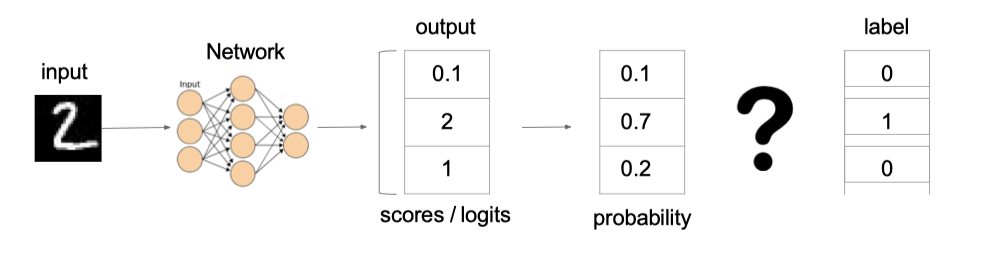
上图中的交叉熵损失为:
$\(-(0log(0.10) + 1log(0.70) + 0log(0.2)) = -log(0.7)\)$
从概率角度理解,我们的目的是最小化正确类别所对应的预测概率的对数的负值(损失值最小),如下图所示:
# 绘制 y=-log(x) 曲线
x = np.linspace(1e-4, 1, 100)  # 避
y = -np.log(x)
# 设置x刻度为0到1
plt.xticks(np.arange(0, 1.1, 0.1))
plt.yticks(np.arange(0, 10, 1))
# 设置坐标轴标签
plt.xlabel("正确类别的预测概率")
plt.ylabel("损失值")
plt.plot(x, y, label="y=-log(x)")
plt.grid(True)
plt.title("多分类交叉熵CrossEntropyLoss")
plt.tight_layout()
plt.legend()
plt.show()
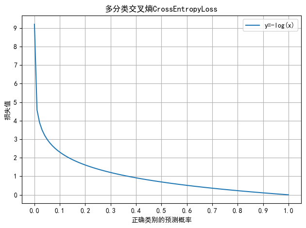
"""
案例:
    演示 多分类交叉熵损失函数

介绍:
    损失函数 也叫 成本函数,目标函数,代价函数,误差函数,用来 衡量模型好坏,也就是模型预测表现
    分类问题:
        多分类交叉熵损失CrossEntropyLoss

多分类交叉熵损失CrossEntropyLoss
    公式:CrossEntropyLoss = -Σylog(S(f(x)))
    其中,x: 样本,f(x): 模型预测的原始输出logits,S(f(x)): 模型预测的概率分布,y:样本x属于某个类别的 真实概率,比如[0,0,1]
    注意:
        CrossEntropyLoss内部进行了Softmax运算,模型输出层无需进行softmax运算,除非在新的数据上预测类别,需要获取预测概率,则需要在模型的原始输出logits上进行softmax

"""

# 导包
import torch
# 1.定义函数,演示 多分类交叉熵损失函数
def demo01():
    # 1.创建 样本的真实类别,针对一个三分类任务,3个样本,真实类别为0,0,1
    # 1.1 使用 one-hot 编码
    # y_true = torch.tensor([[1,0,0],[1,0,0],[0,1,0]], dtype=torch.float)
    # 1.2 使用label编码
    y_true = torch.tensor([0,0,1])
    # 2.创建 模型预测的原始输出logits
    y_logits = torch.tensor([[1.5,0.2,0.9],[0.1,2,0.9],[0.1,0.2,9.4]], requires_grad=True)
    # 3.创建多分类交叉熵损失函数对象
    loss_fn = torch.nn.CrossEntropyLoss()
    # 4.计算损失值
    loss = loss_fn(y_logits,y_true)
    print(f"损失值:{loss}")


# 测试
if __name__ == '__main__':
    demo01()
损失值:4.03115177154541
二分类交叉熵损失 - nn.BCELoss()
二分类任务中可以使用二分类交叉熵损失函数 和 sigmoid
公式为:
$\(loss = -y \log(\hat{y}) - (1-y)\log(1-\hat{y})\)$
其中:
-
y 是样本x属于某一个类别的真实概率
-
而 \(\hat{y}\) 是样本属于某一类别的预测概率
-
loss用来衡量真实值 y 与预测值 \(\hat{y}\) 之间差异的损失函数
# 绘制 y = -log(x), y=-log(1-x)
x = np.linspace(1e-3, 1, 1000)  # 避免对数函数的零值
y1 = -np.log(x)
y2 = -np.log(1 - x)
plt.figure(figsize=(8, 6))
plt.xticks(np.arange(0, 1.1, 0.1))
plt.yticks(np.arange(0, 10, 1))
plt.xlabel("预测概率")
plt.ylabel("损失值")
plt.plot(x, y1, color='blue', label='y=-log(x), 正类样本')
plt.plot(x, y2, color='red', label='y=-log(1-x), 负类样本')
plt.grid(True)
plt.title("二分类交叉熵BCELoss")
plt.legend()
plt.tight_layout()
plt.show()
C:\Users\angmi\AppData\Local\Temp\ipykernel_7796\193180856.py:4: RuntimeWarning: divide by zero encountered in log
  y2 = -np.log(1 - x)
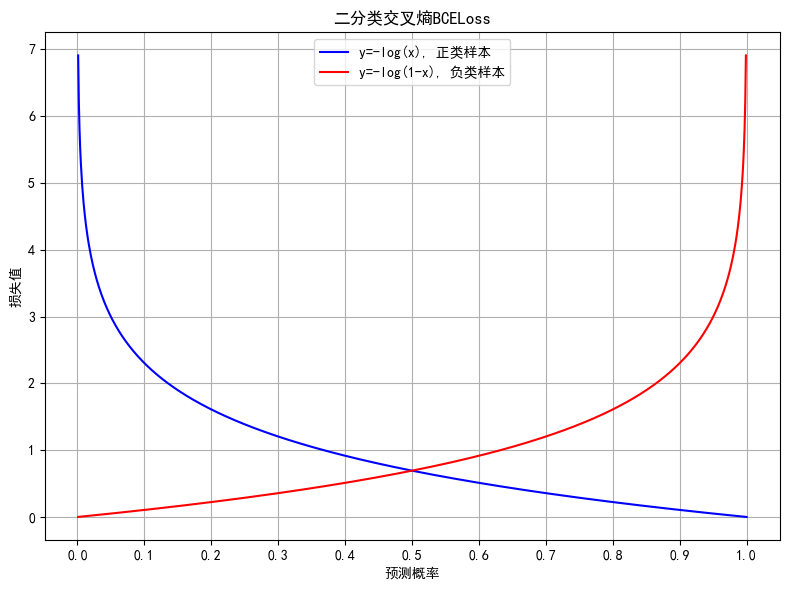
针对二分类问题,CrossEntropyLoss(softmax) 和 BCELoss(sigmoid) 可以互相转化
"""
案例:
    演示 二分类交叉熵损失函数
介绍:
    损失函数 也叫 成本函数,目标函数,代价函数,误差函数,用来 衡量模型好坏,模型预测表现
    分类问题:
        多分类交叉熵损失CrossEntropyLoss
        二分类交叉熵损失BCELoss
多分类交叉熵损失CrossEntropyLoss
    公式:CrossEntropyLoss = -Σylog(S(f(x)))
    其中,x: 样本,f(x): 模型预测的原始输出logits,S(f(x)): 模型预测的概率分布,y:样本x属于某个类别的 真实概率,比如[0,0,1]
    注意:
        CrossEntropyLoss内部进行了Softmax运算,模型输出层无需进行softmax运算,除非在新的数据上预测类别,需要获取预测概率,则需要在模型的原始输出logits上进行softmax

二分类交叉熵损失BCELoss
    公式:BCELoss = -ylog(y_hat)-(1-y)log(1-y_hat)
    注意:
        BCELoss内部没有进行sigmoid运算,使用BCELoss时,模型输出层需要手动添加sigmoid

针对二分类问题,CrossEntropyLoss 和 BCELoss 可以互相转化
注意正类的人为设定,会影响BCELoss 和 CrossEntropyLoss 中 logits的 转换关系
"""


# 导包
import torch
import torch.nn as nn

# 定义函数,演示 二分类交叉熵损失
def demo01():
    print("二分类交叉熵损失")
    # 1. 创建 样本的真实类别, [正,正,负]
    y_true = torch.tensor([1, 1, 0], dtype=torch.float)

    # 2.创建 模型预测 的原始输出logits值
    y_logits = torch.tensor([1,-4,3], dtype=torch.float)
    # sigmoid=1/(1+exp(-x))
    # 经过sigmoid,转化为正类别的 概率
    y_pred = torch.sigmoid(y_logits)
    print(f"y_pred: {y_pred}")

    # 3.创建 交叉熵损失函数
    loss_fn = nn.BCELoss()

    # 4.计算损失
    loss = loss_fn(y_pred, y_true)
    print(f"loss: {loss}")


# 定义函数,演示 多分类交叉熵损失
def demo02():
    print("多分类交叉熵损失")
    # 1. 创建 样本的真实类别, [正,正,负]
    y_true = torch.tensor([1, 1, 0])

    # 2.创建 模型预测 的原始输出logits值
    y_pred = torch.tensor([[2,3], [5,1],[1, 4]], dtype=torch.float)

    # 3.创建 交叉熵损失函数
    loss_fn = nn.CrossEntropyLoss()

    # 4.计算损失
    loss = loss_fn(y_pred, y_true)
    print(f"loss: {loss}")

# 测试
if __name__ == '__main__':
    demo01()
    demo02()
二分类交叉熵损失
y_pred: tensor([0.7311, 0.0180, 0.9526])
loss: 2.4599997997283936
多分类交叉熵损失
loss: 2.4599995613098145
回归任务 - MAE损失函数
mean absolute loss(MAE) 也被称为L1 Loss,计算绝对误差的平均值
损失函数公式:
$\(L = \frac{1}{n}\sum_{i=1}^{n}|y_i - \hat{y}_i|\)$
误差-损失曲线如下图所示:
# 绘制 y=|x|的函数图像
x = np.linspace(-2, 2, 1000)
y = np.abs(x)
plt.figure(figsize=(8, 4))
plt.plot(x, y, label="y=|x|")
# 设置坐标轴标签
plt.xlabel("误差 $y_i - \hat{y}_i$")
plt.ylabel("绝对值")
# 设置刻度
plt.xticks(np.arange(-2, 2.5, 0.5))
plt.yticks(np.arange(0, 2.5, 0.5))
plt.title("L1Loss")
plt.grid()
plt.legend()
plt.tight_layout()
plt.show()
<>:7: SyntaxWarning: invalid escape sequence '\h'
<>:7: SyntaxWarning: invalid escape sequence '\h'
C:\Users\angmi\AppData\Local\Temp\ipykernel_7796\3224521475.py:7: SyntaxWarning: invalid escape sequence '\h'
  plt.xlabel("误差 $y_i - \hat{y}_i$")
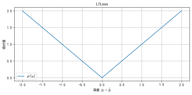
特点是:
- L1 loss具有稀疏性,可以惩罚较大的值,常常作为正则项添加到其他loss中作为约束。(导数恒定为 1或-1,0点不可导, 产生稀疏矩阵)
- L1 loss的最大问题是梯度在零点不平滑,导致会跳过极小值
- 适用于回归问题中存在异常值或噪声数据时,可以减少对离群点的敏感性
# 定义变量,记录 真实值
y_true = torch.tensor([2.0,2.5,3.0], dtype=torch.float)
# 定义变量,记录 预测值
y_pred = torch.tensor([1.5,2.0,2.5], dtype=torch.float, requires_grad=True)
# 创建损失函数,MAE
loss_fn = nn.L1Loss()
# loss_fn = nn.MSELoss()
# loss_fn = nn.SmoothL1Loss()
# 计算损失值
loss = loss_fn(y_pred, y_true)
# 打印损失值
print(f"MAE: {loss}")
MAE: 0.5
回归任务 - MSE损失函数
Mean Squared Loss/ Quadratic Loss(MSE loss) 也被称为L2 loss,或欧氏距离,计算误差平方的平均值
公式:
$\(L = \frac{1}{n}\sum_{i=1}^{n}(y_i - \hat{y}_i)^2\)$
误差-损失曲线如下图所示:
# 绘制 y=x^2 的函数图像
x = np.linspace(-2, 2, 1000)
y = x ** 2
plt.figure(figsize=(8, 7))
plt.plot(x, y, label="y=x^2")
# 设置坐标轴标签
plt.xlabel("误差 $y_i - \hat{y}_i$")
plt.ylabel("平方")
# 设置刻度
plt.xticks(np.arange(-2, 2.5, 0.5))
plt.yticks(np.arange(0, 4.5, 0.5))
plt.title("MSELoss")
plt.grid()
plt.legend()
plt.tight_layout()
plt.show()
<>:7: SyntaxWarning: invalid escape sequence '\h'
<>:7: SyntaxWarning: invalid escape sequence '\h'
C:\Users\angmi\AppData\Local\Temp\ipykernel_7796\1418239404.py:7: SyntaxWarning: invalid escape sequence '\h'
  plt.xlabel("误差 $y_i - \hat{y}_i$")
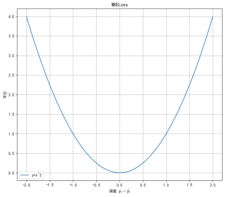
特点是:
- L2 loss也常常作为正则项,对于离群点(outliers)敏感,因为平方项会放大大误差
- 当预测值与目标值相差很大时, 梯度容易爆炸
-
梯度爆炸:网络层之间的梯度(值大于1.0)重复相乘导致的指数级增长
-
适用于大多数标准回归问题,如房价预测、温度预测等
# 定义变量,记录 真实值
y_true = torch.tensor([2.0,2.5,3.0], dtype=torch.float)
# 定义变量,记录 预测值
y_pred = torch.tensor([1.5,2.0,2.5], dtype=torch.float, requires_grad=True)
# 创建损失函数,MSE
# loss_fn = nn.L1Loss()
loss_fn = nn.MSELoss()
# loss_fn = nn.SmoothL1Loss()
# 计算损失值
loss = loss_fn(y_pred, y_true)
# 打印损失值
print(f"MSE: {loss}")
MSE: 0.25
回归任务 - Smooth L1 Loss (也称为 Huber Loss)
Smooth L1 损失函数结合了 MAE 和 MSE,适用于回归任务,尤其是在面对异常值时,它能平滑过渡,避免大误差的影响。
公式如下:
其中:
- \(x_i = y_{\text{pred}, i} - y_{\text{true}, i}\)
- \(n\) 是样本数量
- \(x_i\) 是每个样本的预测误差
解释:
- 当误差 \(|x_i|\) 小于 1 时,使用 L2 损失(平方误差),这意味着损失的增长是 二次方,避免了在训练过程中使用绝对误差导致的梯度不连续问题。
- 当误差 \(|x_i|\) 大于或等于 1 时,使用 L1 损失(绝对误差),避免了大误差对梯度的影响,避免了MSE对离群点过度敏感,可以减少梯度爆炸。
这种方式使得 Smooth L1 Loss 在小误差时更精确,在大误差时能较为稳健地优化。
Smooth L1损失函数图像为:
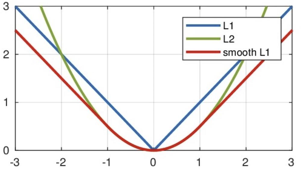
从上图中可以看出,该函数实际上就是一个分段函数
- 在[-1,1]之间实际上就是L2损失,这样解决了L1的不光滑问题
- 在[-1,1]区间外,实际上就是L1损失,这样就解决了离群点梯度爆炸的问题
# 定义变量,记录 真实值
y_true = torch.tensor([2.0,2.5,3.0], dtype=torch.float)
# 定义变量,记录 预测值
y_pred = torch.tensor([1.5,2.0,2.5], dtype=torch.float, requires_grad=True)
# 创建损失函数,SmoothL1Loss
# loss_fn = nn.L1Loss()
# loss_fn = nn.MSELoss()
loss_fn = nn.SmoothL1Loss()
# 计算损失值
loss = loss_fn(y_pred, y_true)
# 打印损失值
print(f"SmoothL1Loss: {loss}")
SmoothL1Loss: 0.125
5.神经网络优化方法
多层神经网络的学习能力比单层网络强得多。想要训练多层网络,需要更强大的学习算法。误差反向传播算法(Back Propagation)是其中最杰出的代表,它是目前最成功的神经网络学习算法。现实任务使用神经网络时,大多是在使用 BP 算法进行训练,值得指出的是 BP 算法不仅可用于多层前馈神经网络,还可以用于其他类型的神经网络。通常说 BP 网络时,一般是指用 BP 算法训练的多层前馈神经网络。
这就需要了解两个概念:
- 正向传播:指的是数据通过网络从输入层到输出层的传递过程。这个过程的目的是计算网络的输出值(预测值),从而与目标值(真实值)比较以计算误差。
- 反向传播:指的是计算损失函数相对于网络中各参数(权重和偏置)的梯度,指导优化器更新参数,从而使神经网络的预测更接近目标值。
6. 梯度下降法
梯度下降法就是一种寻找损失函数最小值的方法。从数学角度来看,梯度的方向是函数增长速度最快的方向,梯度的反方向就是函数减少最快的方向。
基本步骤
- 初始化参数
- 前向传播计算损失
- 反向传播计算梯度
- 更新参数:
$\(w = w - \alpha * \frac{\partial L}{\partial w}\)$
其中\(\alpha\)是学习率。如果学习率太小,那么每次训练之后得到的参数更新效果都太小,增大训练的时间成本。如果,学习率太大,那就有可能直接跳过最优解,进入无限的训练中。解决的方法是,学习率也需要随着训练的进行而变化。
\(\frac{\partial L}{\partial w}\) 是损失函数对模型参数的梯度。

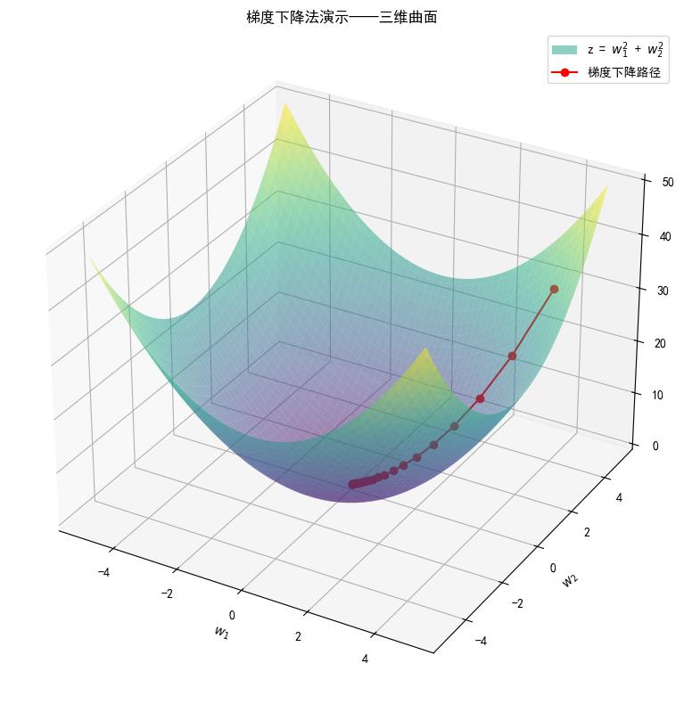
在上图中我们展示了一维和多维的损失函数,损失函数呈碗状。在训练过程中损失函数对权重的偏导数就是损失函数在该位置的梯度。可以看到,沿着负梯度方向移动,就可以到达损失函数底部,从而使损失函数最小化。这种利用损失函数的梯度迭代地寻找最小值的过程就是梯度下降的过程。
在进行模型训练时,有三个基础的概念:
- Epoch: 训练轮数,使用全部数据对模型进行此轮完整训练,比如
Epochs = 100 - Batch: 批次大小,使用训练集中的小部分样本的梯度对模型权重进行更新,比如
batch_size=16 - Iteration: 每次训练的批次数,使用一个 Batch 数据对模型进行一次参数更新的过程,比如
iterations=7
假设数据集有 50000 个训练样本,现在选择 Batch Size = 256 对模型进行训练。
- 每个 Epoch 要训练的图片数量:50000
- 训练集具有的 Batch 个数:(50000-1)//256+1=196
- 每个 Epoch 具有的 Iteration 个数:196
- 10个 Epoch 具有的 Iteration 个数:1960
在深度学习中,梯度下降的几种方式的根本区别就在于Batch Size不同,如下表所示:
| 梯度下降方式 | Training Set Size | Batch Size | Number of Batches |
|--------------|-------------------|------------|-------------------|
| BGD | \(N\) | \(N\) | \(1\) |
| SGD | \(N\) | \(1\) | \(N\) |
| Mini-Batch | \(N\) | \(B\) | $ (N-1)//B + 1 $ |
演示梯度下降法
# 目标函数 & 导数
def f(x):
    return x**2 + 20

def grad(x):
    return 2 * x

# 准备绘图
x_vals = np.linspace(-10, 10, 200)
y_vals = f(x_vals)

plt.figure(figsize=(10,6))
plt.title("梯度下降法演示-二维曲线")
plt.plot(x_vals,y_vals, label="y = $w^{2}$ + 20")
plt.grid()
plt.legend()
plt.tight_layout()
plt.show()

# 梯度下降参数
lr = 0.2          # learning rate
x = -8            # 初始点
steps = 20        # 迭代次数

xs = [x]          # 保存每一步的 x
ys = [f(x)]       # 保存每一步的 y

# 梯度下降过程
for i in range(steps):
    g = grad(x)
    x = x - lr * g
    xs.append(x)
    ys.append(f(x))

# 绘制函数曲线
plt.figure(figsize=(10,6))
plt.plot(x_vals, y_vals, label=r"y = $w^{2}$ + 20")

# 绘制梯度下降路径
plt.scatter(xs, ys, color='red', s=30, label="梯度下降路径")
plt.plot(xs, ys, color='red', linestyle='--')

# 最终点标注
plt.scatter(xs[-1], ys[-1], color='green', s=60, label="最低点")

plt.grid()
plt.legend()
plt.title("梯度下降法演示-二维曲线")
plt.xlabel("w")
plt.ylabel("y")
plt.tight_layout()
plt.show()
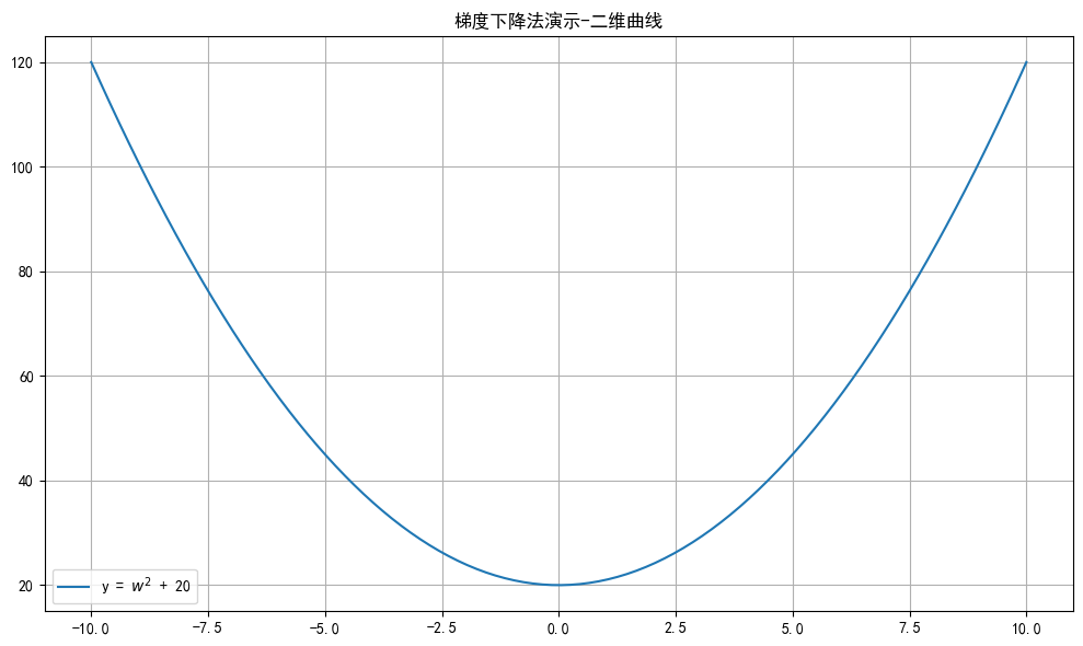
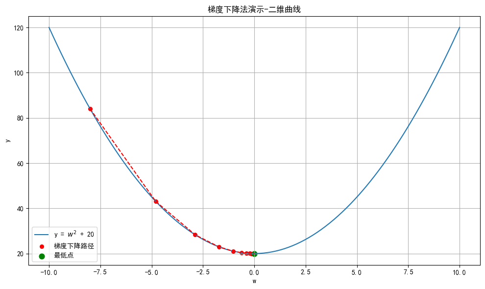
import numpy as np
from mpl_toolkits.mplot3d import Axes3D

# 定义函数及梯度
def f(x, y):
    return x**2 + y**2

def grad_f(x, y):
    return np.array([2*x, 2*y])

# 创建网格
x = np.linspace(-5, 5, 100)
y = np.linspace(-5, 5, 100)
X, Y = np.meshgrid(x, y)
Z = f(X, Y)

# 梯度下降初始化
lr = 0.1  # 学习率
steps = 25
point = np.array([4.0, 4.0])  # 起点
trajectory = [point.copy()]

# 梯度下降迭代
for _ in range(steps):
    grad = grad_f(point[0], point[1])
    point -= lr * grad
    trajectory.append(point.copy())

trajectory = np.array(trajectory)
Z_traj = f(trajectory[:,0], trajectory[:,1])

# 绘图
# Plot surface
fig = plt.figure(figsize=(12,8))
ax = fig.add_subplot(111, projection='3d')
ax.set_title("梯度下降法演示——三维曲面")
ax.plot_surface(X, Y, Z, alpha=0.5, cmap='viridis', label="z = $w_1^{2}$ + $w_2^{2}$")  # No colors specified
ax.set_xlabel(r"$w_1$")
ax.set_ylabel(r"$w_2$")
ax.legend()
plt.tight_layout()

fig = plt.figure(figsize=(12,8))
ax = fig.add_subplot(111, projection='3d')
ax.set_title("梯度下降法演示——三维曲面")
ax.plot_surface(X, Y, Z, alpha=0.5, cmap='viridis', label="z = $w_1^{2}$ + $w_2^{2}$")  # 半透明曲面
ax.plot(trajectory[:,0], trajectory[:,1], Z_traj, color='r', marker='o', label='梯度下降路径')

ax.set_xlabel(r"$w_1$")
ax.set_ylabel(r"$w_2$")
# ax.set_zlabel(r"z = $w_1^{2}$ + $w_2^{2}$")
ax.legend()
plt.tight_layout()
plt.show()
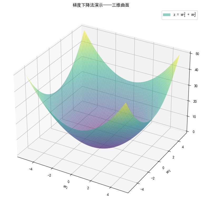
7.反向传播(BP算法)
利用反向传播算法对神经网络进行训练。该方法与梯度下降算法相结合,对网络中所有权重计算损失函数的梯度,并利用梯度值来更新权值以最小化损失函数。
概念
前向传播:数据输入到神经网络中,逐层向前传播,一直运算到输出层为止, 输出预测值。
反向传播(Back Propagation):利用损失函数loss值,从后往前,依次求各个参数的偏导,结合梯度下降算法,更新模型参数。

在网络的训练过程中经过前向传播得到的最终结果跟训练样本的真实值总是存在一定误差,这个误差便是损失函数 ERROR。想要减小这个误差,就用损失函数 ERROR,从后往前,依次求各个参数的偏导,这就是反向传播(Back Propagation), 然后用损失梯度来更新模型参数来减小损失值。
详解
反向传播算法利用链式求导法则对神经网络中的各个节点的权重进行求导运算。
【举个栗子🌰:】
下图是一个简单的神经网络示例:激活函数为sigmoid
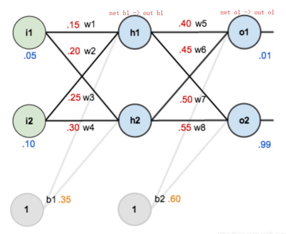
前向传播运算:
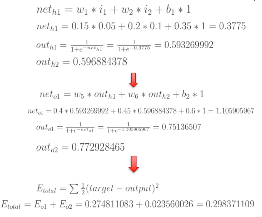
反向传播运算(求损失函数对各个模型参数的梯度):
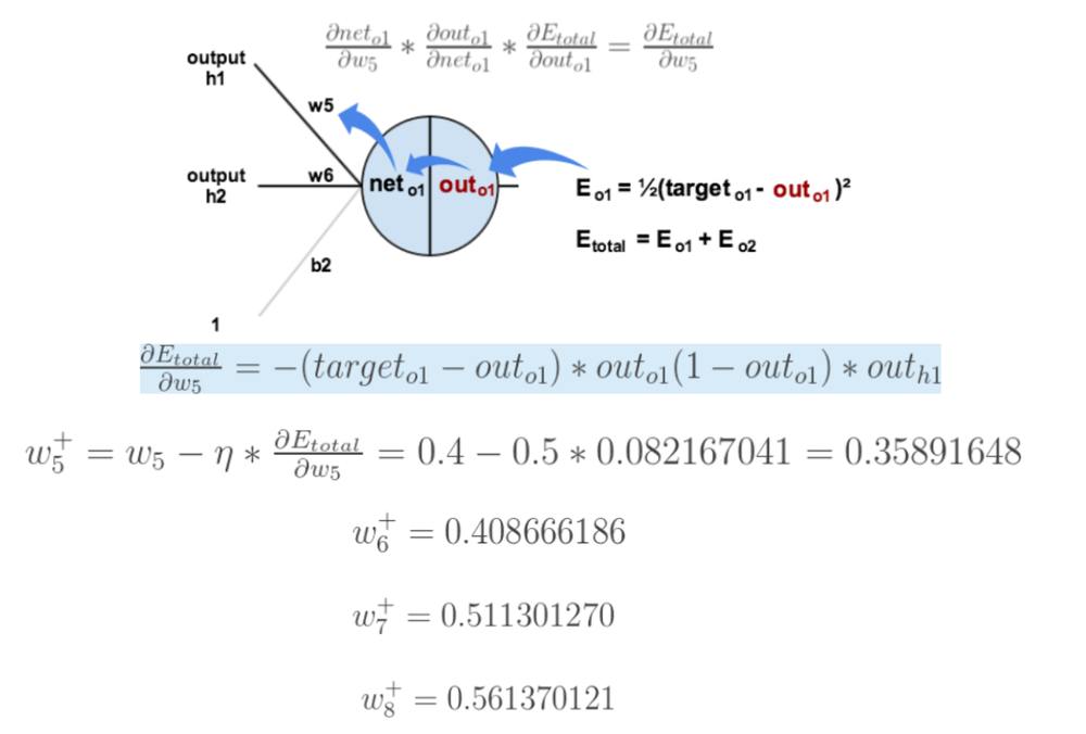
先来求损失函数E对\(w_{5}\)的导数。根据链式求导法则,损失函数E对\(w_{5}\)的导数为:
如下图所示:
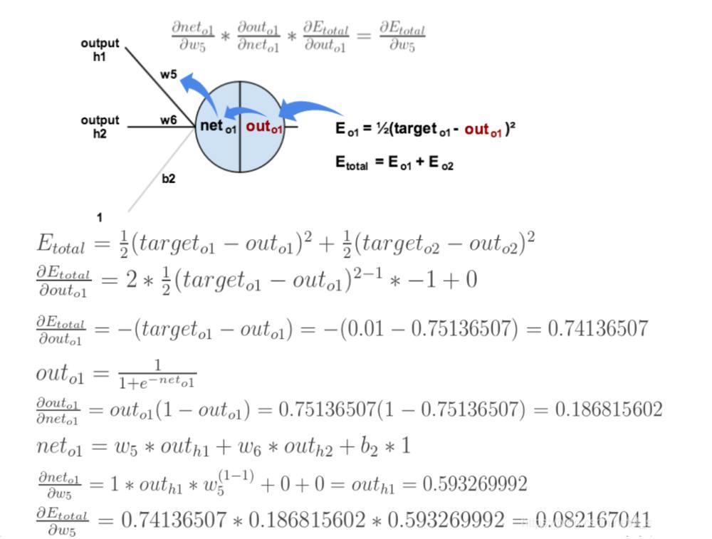
导数(梯度)已经计算出来了,下面就是更新参数过程:
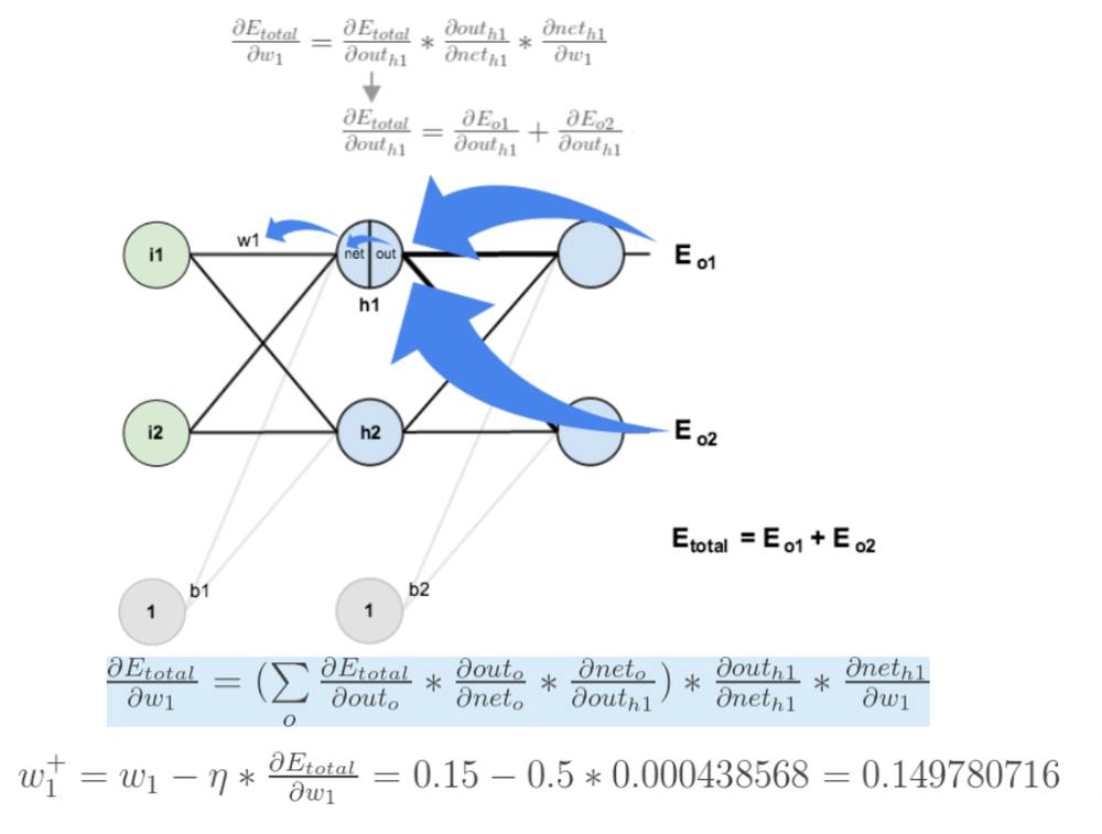
损失函数E对\(w_{1}\)的导数,损失函数E对\(w_{1}\)的求导路径不止一条,这会稍微复杂一点,但换汤不换药,计算过程如下所示:
8.梯度下降优化方法
梯度下降优化算法中,可能会碰到以下情况:
- 碰到平缓区域,梯度值较小,参数优化变慢
- 碰到 “鞍点” ,梯度为0,参数无法优化
- 碰到局部最小值,参数不是最优
对于这些问题, 出现了一些对梯度下降算法的优化方法,例如:Momentum、AdaGrad、RMSprop、Adam 等

指数加权平均
常见的算数平均指的是将所有数加起来除以数的个数,每个数的权重是相同的。指数加权平均指的是给每个数赋予不同的权重求平均数。移动平均数,指的是计算最近邻的 N 个数来获得平均数。
指数移动加权平均则是参考各数值,并且各数值的权重都不同,距离越远的数字对平均数计算的贡献越小(权重较小),距离越近则对平均数计算的贡献越大(权重越大)。
比如:明天气温怎么样,和昨天气温有很大关系,而和一个月前的气温关系就小一些。
计算公式可以用下面的式子来表示:
- \(S_t\) 表示指数加权平均值;
- \(Y_t\) 表示t时刻的值;
- β 调节权重系数,该值越大平均数越平缓。
举个例子,假设 权重 \(\beta\) 为 0.9,则:
- $S_0 = Y_0 $
- \(S_1 = 0.9 \times S_0 + 0.1 \times Y_1\)
- \(S_2 = 0.9 \times S_1 + 0.1 \times Y_2 = 0.9^2 \times Y_0 + 0.9 \times 0.1 \times Y_1 + 0.1 \times Y_2\)
- \(S_3 = 0.9 \times S_2 + 0.1 \times Y_3 = 0.9^3 \times Y_0 + 0.9^2 \times 0.1 \times Y_1 + 0.9 \times 0.1 \times Y_2 + 0.1 \times Y_3\)
- ...
-
\(S_n = 0.9 \times S_{n-1} + 0.1 \times Y_n = 0.9^{n} \times Y_0 + 0.9^{n-1} \times 0.1 \times Y_1 + \dots + 0.9 \times 0.1 \times Y_{n-1} + 0.1 \times Y_n\)
-
$S_{100} = 0.9 \times S_{99} + 0.1 \times Y_{100} = 0.9^{100} \times Y_0 + 0.9^{99} \times 0.1 \times Y_1 + \dots + 0.9 \times 0.1 \times Y_{99} + 0.1 \times Y_{100} $
结论
1. \(S_n\)是 \([Y_0, Y_1, Y_2, ..., Y_n]\) 的加权求和结果 — 指数加权平均值
2. 离当前值\(S_n\)越近的数据,系数越大
"""
案例:
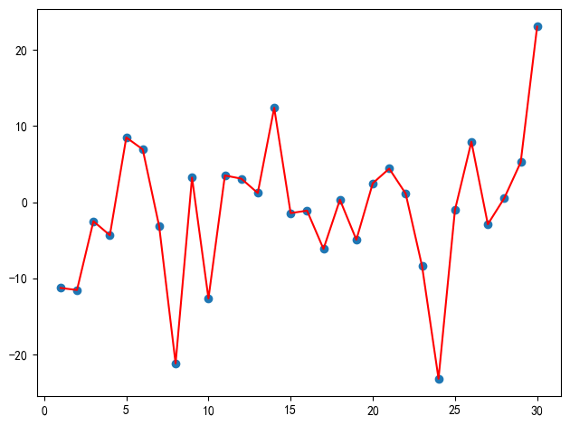
    演示 移动加权平均,使用近30天的天气温度数据.

结论:
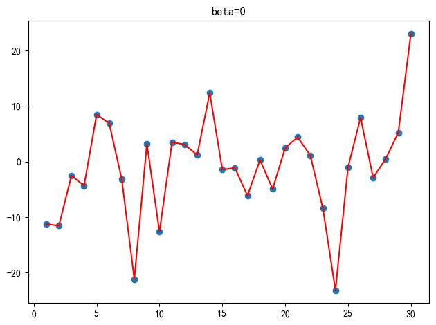
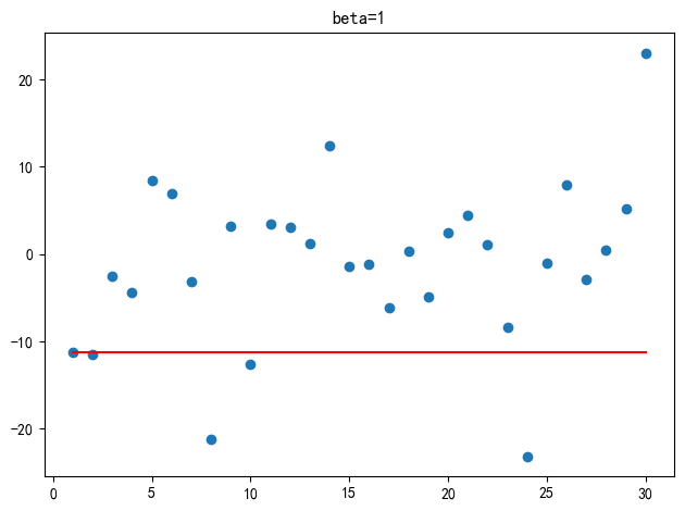
    对于移动加权平均, β值(调节权重系数)越大,移动加权平均值就越依赖历史数据;
    反之,β值(调节权重系数)越小,移动加权平均值就越依赖当天的数据。
    极端情况:β=1,移动加权平均值 = 第一天的数据;β=0,移动加权平均值 = 当天的数据。
"""

import torch
import matplotlib.pyplot as plt

ELEMENT_NUMBER = 30

# 1. 实际平均温度
def demo01():
    # 固定随机数种子
    torch.manual_seed(0)
    # 产生30天的随机温度
    temperature = torch.randn(size=[ELEMENT_NUMBER, ]) * 10
    print(temperature)
    # 绘制平均温度
    days = torch.arange(1, ELEMENT_NUMBER + 1, 1)
    plt.plot(days, temperature, color='r')
    plt.scatter(days, temperature)
    plt.tight_layout()
    plt.show()


# 2. 指数加权平均温度
def demo02(beta=0.9):
    # 固定随机数种子,确保每次运行得到相同的随机温度数据
    torch.manual_seed(0)
    # 产生30天的随机温度数据,通过乘以10放大温度范围
    temperature = torch.randn(size=[ELEMENT_NUMBER, ]) * 10
    print(temperature)

    # 存储指数加权平均后的温度值
    exp_weight_avg = []
    # 遍历每天的温度数据,idx从0开始计数
    for idx, temp in enumerate(temperature):
        # 第一天的指数加权平均值就是当天温度本身
        if idx == 0:
            exp_weight_avg.append(temp)
            continue
        # 从第二天开始,按照指数加权平均公式计算:
        # V_t = β * V_{t-1} + (1-β) * θ_t
        # 其中 V_t 是当前时刻的加权平均值,V_{t-1} 是上一时刻的加权平均值
        # θ_t 是当前时刻的实际温度值,β 是权重参数(0<=β<1)
        # idx-1 是因为要访问前一天的加权平均值
        new_temp = exp_weight_avg[idx - 1] * beta + (1 - beta) * temp
        exp_weight_avg.append(new_temp)

    # 创建天数序列用于绘图
    days = torch.arange(1, ELEMENT_NUMBER + 1, 1)
    # 设置图表标题,显示当前使用的beta值
    plt.title(f"beta={beta}")
    # 绘制指数加权平均温度曲线(红色)
    plt.plot(days, exp_weight_avg, color='r')
    # 绘制原始温度数据点
    plt.scatter(days, temperature)
    plt.tight_layout()
    # 显示图表
    plt.show()


if __name__ == '__main__':
    demo01()
    demo02(0)
    demo02(0.5)
    demo02(0.9)
    demo02(1)
tensor([-11.2584, -11.5236,  -2.5058,  -4.3388,   8.4871,   6.9201,  -3.1601,
        -21.1522,   3.2227, -12.6333,   3.4998,   3.0813,   1.1984,  12.3766,
         -1.4347,  -1.1161,  -6.1358,   0.3159,  -4.9268,   2.4841,   4.3970,
          1.1241,  -8.4106, -23.1604,  -1.0231,   7.9244,  -2.8967,   0.5251,
          5.2286,  23.0221])
tensor([-11.2584, -11.5236,  -2.5058,  -4.3388,   8.4871,   6.9201,  -3.1601,
        -21.1522,   3.2227, -12.6333,   3.4998,   3.0813,   1.1984,  12.3766,
         -1.4347,  -1.1161,  -6.1358,   0.3159,  -4.9268,   2.4841,   4.3970,
          1.1241,  -8.4106, -23.1604,  -1.0231,   7.9244,  -2.8967,   0.5251,
          5.2286,  23.0221])
tensor([-11.2584, -11.5236,  -2.5058,  -4.3388,   8.4871,   6.9201,  -3.1601,
        -21.1522,   3.2227, -12.6333,   3.4998,   3.0813,   1.1984,  12.3766,
         -1.4347,  -1.1161,  -6.1358,   0.3159,  -4.9268,   2.4841,   4.3970,
          1.1241,  -8.4106, -23.1604,  -1.0231,   7.9244,  -2.8967,   0.5251,
          5.2286,  23.0221])
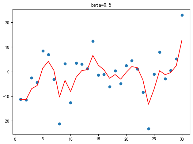
tensor([-11.2584, -11.5236,  -2.5058,  -4.3388,   8.4871,   6.9201,  -3.1601,
        -21.1522,   3.2227, -12.6333,   3.4998,   3.0813,   1.1984,  12.3766,
         -1.4347,  -1.1161,  -6.1358,   0.3159,  -4.9268,   2.4841,   4.3970,
          1.1241,  -8.4106, -23.1604,  -1.0231,   7.9244,  -2.8967,   0.5251,
          5.2286,  23.0221])
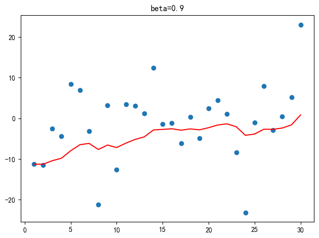
tensor([-11.2584, -11.5236,  -2.5058,  -4.3388,   8.4871,   6.9201,  -3.1601,
        -21.1522,   3.2227, -12.6333,   3.4998,   3.0813,   1.1984,  12.3766,
         -1.4347,  -1.1161,  -6.1358,   0.3159,  -4.9268,   2.4841,   4.3970,
          1.1241,  -8.4106, -23.1604,  -1.0231,   7.9244,  -2.8967,   0.5251,
          5.2286,  23.0221])
动量算法Momentum
当梯度下降碰到 “峡谷” 、”平缓”、”鞍点” 区域时, 参数更新变慢。 Momentum 通过指数加权平均法,累计历史梯度值,进行参数更新,越近的梯度值对当前参数更新的影响越大。
梯度计算公式:
$\(s_t=βs_{t−1}+(1−β)g_t\)$
参数更新公式:
$\(w_t=w_{t−1}−ηs_t\)$
\(s_t\)是当前时刻的梯度的指数移动加权平均值
\(s_{t-1}\)是上一时刻的梯度的指数移动加权平均值
\(g_t\)是当前时刻的梯度值
β 是调节权重系数,通常取 0.9 或 0.99
η是学习率
\(w_t\)是当前时刻模型权重参数
print("梯度下降优化方法 —— 动量法Momentum")
# 1.初始化模型参数w
w = torch.tensor([1.0], requires_grad=True, dtype=torch.float32)
# 2.求损失值
loss = 0.5*(w**2)   # w
# 3.创建优化器,基于SGD, 加入动量 momentum(动量参数),就是动量法
# 参数1:待优化的模型参数列表,参数2:学习率,参数3:动量参数
optimizer = optim.SGD([w], lr=0.01, momentum=0.9)   # momentum默认0,也就是无动量的随机梯度下降法
# 4.计算梯度,梯度清零 + 反向传播 + 更新参数
optimizer.zero_grad()   # 梯度清零
loss.mean().backward()  # 反向传播
optimizer.step()    # 更新参数
print(f"第一次梯度更新结果:\nw:{w}, w.grad: {w.grad}")

# 第二次计算损失值
loss = 0.5 * (w ** 2)  # w
optimizer.zero_grad()   # 梯度清零
loss.mean().backward()  # 反向传播
optimizer.step()    # 更新参数
print(f"第二次梯度更新结果:\nw:{w}, w.grad: {w.grad}")
梯度下降优化方法 —— 动量法Momentum
第一次梯度更新结果:
w:tensor([0.9900], requires_grad=True), w.grad: tensor([1.])
第二次梯度更新结果:
w:tensor([0.9711], requires_grad=True), w.grad: tensor([0.9900])
- Momentum 理论公式 vs SGD-Momentum 真实公式
| 方面 | 理论公式 (Classical Momentum) | 框架公式 (PyTorch SGD-Momentum) |
|---|---|---|
| 动量计算 | \(s_t = \beta s_{t-1} + (1-\beta) g_t\) | \(s'_t = \beta s'_{t-1} + \eta g_t\) , 等价于\(s_t = \beta s_{t-1} + g_t\) |
| 参数更新 | \(w_t = w_{t-1} - \eta s_t\) | \(w_t = w_{t-1} - s'_t\) |
| 梯度定义 | \(g_t = \nabla L(w_{t-1})\) | \(g_t = \nabla L(w_{t-1})\) |
| 动量定义 | \(s_t\) 为累积梯度(速度) | \(s'_t = \eta s_t\) 已包含学习率 |
| 说明 | 学习率在参数更新时乘 | 学习率提前合并到动量计算中,更新直接减去 \(s'_t\) |
区别:框架公式的动量计算中,取消了\((1-\beta)\)缩放。
详细解释计算逻辑
w_init = 1.0
momentum = 0.9
lr = 0.01
# 计算梯度
g0 = w_init # 1.0
# 计算s0
s0 = 0 + lr*g0 # 0.01*1.0
# 计算w0
w0 = w_init - s0 # 1.0 - 0.01*1.0 = 0.99
print(f"第一次更新参数之后:w0: {w0}, g0: {g0}")
# 计算g1
g1 = w0 # 0.99
# 计算s1
s1 = momentum * s0 + lr * g1 # 0.9*0.01 + 0.01*0.99 = 0.009+0.0099 = 0.0189
# 计算w1
w1 = w0 - s1    # 0.99 - 0.0189 = 0.9711
print(f"w1: {w1}, g1: {g1}")
第一次更新参数之后:w0: 0.99, g0: 1.0
w1: 0.9711, g1: 0.99
AdaGrad
通过对不同的参数分量使用不同的学习率,AdaGrad 的学习率总体会逐渐减小,AdaGrad 认为:在起初时,我们距离最优目标仍较远,可以使用较大的学习率,加快训练速度,随着迭代次数的增加,学习率逐渐下降。
其计算步骤如下:
-
初始化学习率 η、初始化参数w、小常数 \(σ = 1e-10\)
-
初始化梯度累计变量 s = 0
- 从训练集中采样 m 个样本的小批量,计算梯度\(g_t\)
-
累积平方梯度,⊙ 表示各个分量相乘, 公式为:
$\(s_t = s_{t-1} + g_t⊙g_t\)$
-
学习率 η 的计算公式如下:
-
权重参数更新公式如下:
$\(w_t = w_{t-1} - \frac{η}{\sqrt{s_t}+σ} * g_t\)$
-
重复 3-7 步骤
AdaGrad 缺点是可能会使得学习率过早、过量的降低,导致模型训练后期学习率太小,较难找到最优解。
print("梯度下降优化方法 —— adagrad")
# 1.初始化模型参数w
w = torch.tensor([1.0], requires_grad=True, dtype=torch.float32)
# 2.求损失值
loss = 0.5*(w**2)   # w
# 3.创建优化器,基于SGD, 加入动量 momentum(动量参数),就是动量法
# 参数1:待优化的模型参数列表,参数2:学习率,参数3:动量参数
# optimizer = optim.SGD([w], lr=0.01, momentum=0.9)   # momentum默认0,也就是无动量的随机梯度下降法
# 参数1:待优化的模型参数列表,参数2:学习率
optimizer = optim.Adagrad([w], lr=0.01)
# 4.计算梯度,梯度清零 + 反向传播 + 更新参数
optimizer.zero_grad()   # 梯度清零
loss.mean().backward()  # 反向传播
optimizer.step()    # 更新参数
print(f"第一次梯度更新结果:\nw:{w}, w.grad: {w.grad}")

# 第二次计算损失值
loss = 0.5 * (w ** 2)  # w
optimizer.zero_grad()   # 梯度清零
loss.mean().backward()  # 反向传播
optimizer.step()    # 更新参数
print(f"第二次梯度更新结果:\nw:{w}, w.grad: {w.grad}")
梯度下降优化方法 —— adagrad
第一次梯度更新结果:
w:tensor([0.9900], requires_grad=True), w.grad: tensor([1.])
第二次梯度更新结果:
w:tensor([0.9830], requires_grad=True), w.grad: tensor([0.9900])
RMSProp
RMSProp 优化算法是对 AdaGrad 的优化。最主要的不同是,其使用指数加权平均梯度替换累计平方梯度。
其计算过程如下:
-
初始化学习率 η、初始化权重参数w、小常数 σ = 1e-10
-
初始化梯度累计变量 s = 0
-
从训练集中采样 m 个样本的小批量,计算梯度 \(g_t\)
-
使用指数加权平均累计历史梯度,⊙ 表示各个分量相乘,公式如下:
$\(s_t = βs_{t-1} + (1-β)g_t⊙g_t\)$
-
学习率 η 的计算公式如下:
- 权重参数更新公式如下:
- 重复 3-7 步骤
RMSProp 与 AdaGrad 最大的区别是对梯度的累积方式不同,对于每个梯度分量仍然使用不同的学习率。
RMSProp 通过引入衰减系数β,控制对历史梯度信息获取的多少. 被证明在神经网络非凸条件下的优化更好,学习率衰减更加合理。
需要注意的是:AdaGrad 和 RMSProp 都是对于不同的参数分量使用不同的学习率,如果某个参数分量的梯度值较大,则对应的学习率就会较小,反之,则对应的学习率就会较大。
print("梯度下降优化方法 —— rmsprop")
# 1.初始化模型参数w
w = torch.tensor([1.0], requires_grad=True, dtype=torch.float32)
# 2.求损失值
loss = 0.5*(w**2)   # w
# 3.创建优化器,基于SGD, 加入动量 momentum(动量参数),就是动量法
# 参数1:待优化的模型参数列表,参数2:学习率,参数3:动量参数
# optimizer = optim.SGD([w], lr=0.01, momentum=0.9)   # momentum默认0,也就是无动量的随机梯度下降法
# 参数1:待优化的模型参数列表,参数2:学习率
# optimizer = optim.Adagrad([w], lr=0.01)
# 参数1:待优化的模型参数列表,参数2:学习率,参数3:调和权重系数
optimizer = optim.RMSprop([w], lr=0.01, alpha=0.99)
# 4.计算梯度,梯度清零 + 反向传播 + 更新参数
optimizer.zero_grad()   # 梯度清零
loss.mean().backward()  # 反向传播
optimizer.step()    # 更新参数
print(f"第一次梯度更新结果:\nw:{w}, w.grad: {w.grad}")

# 第二次计算损失值
loss = 0.5 * (w ** 2)  # w
optimizer.zero_grad()   # 梯度清零
loss.mean().backward()  # 反向传播
optimizer.step()    # 更新参数
print(f"第二次梯度更新结果:\nw:{w}, w.grad: {w.grad}")
梯度下降优化方法 —— rmsprop
第一次梯度更新结果:
w:tensor([0.9000], requires_grad=True), w.grad: tensor([1.])
第二次梯度更新结果:
w:tensor([0.8329], requires_grad=True), w.grad: tensor([0.9000])
Adam
-
Momentum 使用指数加权平均计算当前的梯度值
-
AdaGrad、RMSProp 使用自适应的学习率
-
Adam优化算法(Adaptive Moment Estimation,自适应矩估计)将 Momentum 和 RMSProp 算法结合在一起
- 修正梯度: 使⽤梯度的指数加权平均
-
修正学习率: 使⽤梯度平⽅的指数加权平均
-
原理:Adam 是结合了 Momentum 和 RMSProp 的优点的自适应学习率算法。它计算了梯度的一阶矩(平均值)和二阶矩(梯度的平方)的自适应估计,从而动态调整学习率。
-
梯度计算公式:
$\(m_t=β_1m_{t−1}+(1−β_1)g_t\)$
$\(s_t=β_2s_{t−1}+(1−β_2)g_t^2\)$
$\(\hat{m_t} = \frac{m_t}{1−β_1^t}\)$
$\(\hat{s_t}=\frac{s_t}{1−β_2^t}\)$
-
权重参数更新公式:
$\(w_t = w_{t−1} − \frac{η}{\sqrt{\hat{s_t}}+ϵ}\hat{m_t}\)$
其中,\(m_t\) 是梯度的一阶矩估计,\(s_t\) 是梯度的二阶矩估计,\(\hat{m_t}\) 和 \(\hat{s_t}\) 是偏差校正后的估计。
print("梯度下降优化方法 —— adam")
# 1.初始化模型参数w
w = torch.tensor([1.0], requires_grad=True, dtype=torch.float32)
# 2.求损失值
loss = 0.5*(w**2)   # w
# 3.创建优化器,基于SGD, 加入动量 momentum(动量参数),就是动量法
# 参数1:待优化的模型参数列表,参数2:学习率,参数3:动量参数
# optimizer = optim.SGD([w], lr=0.01, momentum=0.9)   # momentum默认0,也就是无动量的随机梯度下降法
# 参数1:待优化的模型参数列表,参数2:学习率
# optimizer = optim.Adagrad([w], lr=0.01)
# 参数1:待优化的模型参数列表,参数2:学习率,参数3:调和权重系数
# optimizer = optim.RMSprop([w], lr=0.01, alpha=0.99)
optimizer = optim.Adam([w], lr=0.01, betas=(0.9, 0.999), weight_decay=1e-3)
# 4.计算梯度,梯度清零 + 反向传播 + 更新参数
optimizer.zero_grad()   # 梯度清零
loss.mean().backward()  # 反向传播
optimizer.step()    # 更新参数
print(f"第一次梯度更新结果:\nw:{w}, w.grad: {w.grad}")

# 第二次计算损失值
loss = 0.5 * (w ** 2)  # w
optimizer.zero_grad()   # 梯度清零
loss.mean().backward()  # 反向传播
optimizer.step()    # 更新参数
print(f"第二次梯度更新结果:\nw:{w}, w.grad: {w.grad}")
梯度下降优化方法 —— adam
第一次梯度更新结果:
w:tensor([0.9900], requires_grad=True), w.grad: tensor([1.])
第二次梯度更新结果:
w:tensor([0.9800], requires_grad=True), w.grad: tensor([0.9900])
AdamW 优化算法
AdamW(Adam with Weight Decay)是 Adam 优化器的一个变种,它在保持 Adam 优点的同时,修正了权重衰减(Weight Decay)的实现方式,在各种深度学习任务中展现出更好的泛化性能。
与Adam的核心区别:从梯度计算到参数更新
- Adam 的实现方式
梯度计算(权重衰减添加到梯度中):
g_t^{\text{Adam}} = ∇L_{\text{data}}(w_{t-1}) + λ w_{t-1}
权重衰减项 \(λ w_{t-1}\) 被直接添加到梯度中,参与后续的自适应计算。
- AdamW 的实现方式
梯度计算(纯数据梯度):
g_t = ∇L_{\text{data}}(w_{t-1}) \quad
梯度计算不包含权重衰减项。权重衰减在参数更新阶段独立处理。
- AdamW/Adam 共同步骤
梯度矩估计:
m_t = β_1 m_{t−1} + (1 − β_1) g_t
s_t = β_2 s_{t−1} + (1 − β_2) g_t^2
偏差校正:
\hat{m_t} = \frac{m_t}{1 − β_1^t}, \quad \hat{s_t} = \frac{s_t}{1 − β_2^t}
- Adam参数更新 耦合了 权重衰减\(λ w_{t-1}\) 和 梯度的一阶矩\(\hat{m_t}\)与二阶矩\(\hat{s_t}\)
w_t = w_{t−1} - \frac{η}{\sqrt{\hat{s_t}} + ϵ} \hat{m_t}
其中
g_t^{\text{Adam}} = ∇L_{\text{data}}(w_{t-1}) + λ w_{t-1}
- AdamW参数更新:
w_t = (1 - ηλ) w_{t−1} - \frac{η}{\sqrt{\hat{s_t}} + ϵ} \hat{m_t}
- 关键优势
AdamW 通过将权重衰减从梯度计算中解耦,实现了真正的 L2 正则化,训练更稳定,成为现代深度学习特别是 Transformer 模型的首选优化器。
print("梯度下降优化方法 —— adamw")
# 1.初始化模型参数w
w = torch.tensor([1.0], requires_grad=True, dtype=torch.float32)
# 2.求损失值
loss = 0.5*(w**2)   # w
# 3.创建优化器,基于SGD, 加入动量 momentum(动量参数),就是动量法
# 参数1:待优化的模型参数列表,参数2:学习率,参数3:动量参数
# optimizer = optim.SGD([w], lr=0.01, momentum=0.9)   # momentum默认0,也就是无动量的随机梯度下降法
# 参数1:待优化的模型参数列表,参数2:学习率
# optimizer = optim.Adagrad([w], lr=0.01)
# 参数1:待优化的模型参数列表,参数2:学习率,参数3:调和权重系数
# optimizer = optim.RMSprop([w], lr=0.01, alpha=0.99)
optimizer = optim.AdamW([w], lr=0.01, betas=(0.9, 0.999), weight_decay=1e-3)
# 4.计算梯度,梯度清零 + 反向传播 + 更新参数
optimizer.zero_grad()   # 梯度清零
loss.mean().backward()  # 反向传播
optimizer.step()    # 更新参数
print(f"第一次梯度更新结果:\nw:{w}, w.grad: {w.grad}")

# 第二次计算损失值
loss = 0.5 * (w ** 2)  # w
optimizer.zero_grad()   # 梯度清零
loss.mean().backward()  # 反向传播
optimizer.step()    # 更新参数
print(f"第二次梯度更新结果:\nw:{w}, w.grad: {w.grad}")
梯度下降优化方法 —— adamw
第一次梯度更新结果:
w:tensor([0.9900], requires_grad=True), w.grad: tensor([1.])
第二次梯度更新结果:
w:tensor([0.9800], requires_grad=True), w.grad: tensor([0.9900])
| 优化算法 | 核心思想 | 核心变量(递推) | 参数更新 | 典型场景 | PyTorch 示例 |
|---|---|---|---|---|---|
| SGD | 使用当前梯度直接更新参数 | \(g_t = \nabla L(w_{t-1})\) | \(w_t = w_{t-1} - \eta g_t\) | 凸优化、简单模型 | optim.SGD(params, lr=1e-3) |
| Momentum | 累积历史梯度,加速收敛、减小震荡,可能跨过 鞍点 或 局部最小值 | \(g_t = \nabla L(w_{t-1})\) \(s_t = \beta s_{t-1} + (1-\beta) g_t\) |
\(w_t = w_{t-1} - \eta s_t\) | 深层网络 | optim.SGD(params, lr=1e-2, momentum=0.9) |
| AdaGrad | 自适应学习率,可能过早过快的降低学习率 | \(g_t = \nabla L(w_{t-1})\) \(s_t = s_{t-1} + g_t^2\) |
\(w_t = w_{t-1} - \dfrac{\eta}{\sqrt{s_t}+\epsilon} g_t\) | 稀疏特征(NLP) | optim.Adagrad(params, lr=1e-2) |
| RMSProp | 指数移动平均,缓解 AdaGrad 衰减过快,没有调整梯度,可能陷入 鞍点 或 局部最小值 | \(g_t = \nabla L(w_{t-1})\) \(s_t = \beta s_{t-1} + (1-\beta) g_t^2\) |
\(w_t = w_{t-1} - \dfrac{\eta}{\sqrt{s_t}+\epsilon} g_t\) | RNN / 非平稳目标 | optim.RMSprop(params, lr=1e-3) |
| Adam | 同时调整 学习率 和 梯度: 一阶矩(调整梯度) + 二阶矩(调整学习率)自适应优化 | $\(g_t=\nabla L(w_{t-1})+\lambda w_{t-1}\)$ $\(m_t=\beta_1 m_{t-1}+(1-\beta_1)g_t\)$ $\(s_t=\beta_2 s_{t-1}+(1-\beta_2)g_t^2\)$ $\(\hat m_t=\frac{m_t}{1-\beta_1^t}\)$ $\(\hat s_t=\frac{s_t}{1-\beta_2^t}\)$ | \(w_t=w_{t-1}-\dfrac{\eta}{\sqrt{\hat s_t}+\epsilon}\hat m_t\) | 通用深度学习 | optim.Adam(params, lr=1e-3) |
| AdamW | Adam + 解耦权重衰减 | \(g_t=\nabla L(w_{t-1})\) \(m_t,s_t\) 同 Adam |
\(w_t=w_{t-1}-\dfrac{\eta}{\sqrt{\hat s_t}+\epsilon}\hat m_t-\eta\lambda w_{t-1}\) | Transformer / CV / NLP | optim.AdamW(params, lr=1e-3, weight_decay=1e-3) |
-
如何选择:AdamW(首选)/Adam -> SGD/Momentum
-
简单任务和较小的模型:SGD 或 Momentum
-
复杂任务或有大量数据: AdamW(首选)或 Adam,在大部分任务上都表现优秀
常见面试题
1. pytorch神经网络训练中为什么要在反向传播之前进行梯度清零?
因为pytorch默认梯度累加
2. 多分类交叉熵损失函数的公式是什么?
-sum(真实类别*log(softmax(预测分数logits))), 正确类别的预测概率的对数的负数
3. 二分类任务中,使用 多分类交叉熵损失 和 二分类交叉熵损失 时 应该注意哪些,有何区别?
1.多分类交叉熵损失,自带了softmax, 模型输出不需要激活函数
2.二分类交叉熵损失,没有sigmoid,模型输出需要激活函数sigmoid
4. 简述梯度下降法的原理
w新 = w旧 - 学习率 * 梯度(当前批次)
沿着梯度的反方向,更新模型参数
5. 梯度下降法的缺点有哪些?
1.平缓区域,更新慢
2.鞍点,停止更新
3.局部最小值,停止更新
6. 梯度下降法的优化方法有哪些?
动量法,Adagrad, RMSProp, Adam(AdamW)
7. 动量法是如何更新模型参数的?
1.使用梯度的指数移动加权平均来替代梯度
2.w新 = w旧 - 学习率 * st
8. Adam是如何更新模型参数的?
1.使用梯度的一阶矩来修正梯度
2.使用梯度二阶矩来修正学习率
9. 神经网络的反向传播算法是如何求导的?
1.链式法则求导
2.沿着求导路径对模型参数进行链式法则求导之后,然后累加求导结果
1. pytorch神经网络训练中为什么要在反向传播之前进行梯度清零?
- 因为PyTorch默认梯度会累积,如果不清零,多个反向传播梯度会相加,可能导致梯度爆炸或梯度消失,从而影响训练效果。
- 所以在每次反向传播前,需要调用
optimizer.zero_grad()清零梯度。
2. 多分类交叉熵损失函数的公式是什么?
- 公式:\(-\sum 真实类别 \log(预测概率)\),等价于 – log(正确类别的预测概率)。
- 内部已包含 softmax 运算。
3. 二分类任务中,使用 多分类交叉熵损失 和 二分类交叉熵损失 时 应该注意哪些,有何区别?
- 二分类任务,使用多分类交叉熵损失时,需要注意两个方面:
- 1.网络输出层的输出维度为2,分别对应正类别和负类别;
- 2.无需在网络输出层添加softmax,因为多分类交叉熵损失函数内部有softmax运算。
- 使用二分类交叉熵损失时,需要注意两个方面:
- 1.网络输出层的输出维度为1,输出对应正类别概率,负类别概率为1-正类别概率;
- 2.需要在网络输出层添加sigmoid,因为二分类交叉熵损失函数内部没有sigmoid运算。
4.简述梯度下降法的原理
- 梯度下降法的目标是找到损失函数的最小值,从而获取最优的模型参数。
- 具体做法为,首先计算损失函数对模型参数的梯度,然后沿着梯度的反方向迭代更新模型参数,直到找到损失函数的最小值。
- 更新参数的公式为:Wt = Wt-1 - 学习率 * 梯度
5. 梯度下降法的缺点有哪些?
主要有三个:
- 1.碰到小梯度的平缓区域,参数更新变慢;
- 2.碰到0梯度的 “鞍点”,参数无法更新;
- 3.可能陷入局部最小值,训练提前终止
6. 梯度下降法的优化方法有哪些?
- 1.动量法Momentum
- 2.自适应学习率AdaGrad
- 3.RMSProp
- 4.Adam/AdamW
7. 动量法是如何更新模型参数的?
- 动量法Momentum 是一种优化方法,通过引入动量参数,来加速模型参数的更新。
- 动量法Momentum 的更新公式为:
St = β * St-1(上一次) + (1-β) * 梯度(当前),
Wt = Wt-1 - 学习率 * St,
St为梯度的指数加权平均值,β为权重系数,通常为0.9。
8. Adam是如何更新模型参数的?
Adam 是结合 动量法Momentum 和 RMSProp 的自适应优化算法。
- 1.对梯度做一阶矩和二阶矩的指数加权移动平均,得到mt 和 st
- 2.再进行偏差校正得到mt_hat 和 st_hat
- 3.然后按公式 Wt=Wt-1−学习率/(√st_hat + 小常数) * mt_hat,来更新模型参数,从而实现自适应学习率, 并加速收敛。
9. 神经网络的反向传播算法是如何求导的?
- 反向传播通过链式法则在计算图上从输出向输入反向计算梯度。
- 对任意参数,梯度是损失函数到该参数的所有路径的梯度累加,其中每条路径的梯度按链式法则相乘得到。
- 本质上,损失函数对每个参数 w 的梯度是损失函数到参数 \( w \) 的所有路径的链式法则乘积之和:
代码作业
- 1.搭建一个神经网络,有3个隐藏层和1个输出层,输入数据的输入特征维度为20,3个隐藏层的神经元数量分别为128,64,32,输出层的神经元数量为4。激活函数要求为:隐藏层使用relu激活函数,输出层使用softmax激活函数。并打印模型结构 和 模型参数。
- 2.使用代码演示 二分类任务中,分别使用 多分类交叉熵CrossEntropyLoss 和 二分类交叉熵BCELoss,比如原始输出的logits为:两个类别[[3,1], [4,3], [2,4]],单个类别为[2,1,-2],分别计算对应的 多分类交叉熵损失值 和 二分类交叉熵损失值,并打印。
- 3.使用pytorch计算MSE损失值。已知 y_ture 为 [1, 2, 3, 4, 5, 6], y_pred 为 [2, 3, 4, 5, 6, 7],计算MSE损失值,并打印。
- 4.使用梯度下降法,使用optim.SGD实现,循环迭代800次,求 loss = 0.5*w**2 + 10 的极小值点, 并打印loss最小值,以及loss是最小值时 w的值 和 梯度。
- 5.使用Adam优化器,使用optim.Adam实现,循环迭代800次,求 loss = 0.5*w**2 + 10 的极小值点, 并打印loss最小值,以及loss是最小值时 w的值 和 梯度。
- 6.使用AdamW优化器,使用optim.Adamw实现,循环迭代800次,求 loss = 0.5*w**2 + 10 的极小值点, 并打印loss最小值,以及loss是最小值时 w的值 和 梯度。
Day04 代码:激活函数 / 初始化 / 网络搭建
3 个文件- 📄 01_激活函数.py 6.7KB 下载
- 📄 02_演示参数初始化.py 4.1KB 下载
- 📄 03_搭建神经网络.py 2.4KB 下载
论文:Kaiming 初始化
- 📕 kaiming.pdf 2.2MB
📄 kaiming.pdf · 文字提取版
以下为 PDF 文字提取版(排版有简化,原文见附件)。
第 1 页
Delving Deep into Rectifiers: Surpassing Human-Level Performance on ImageNet Classification Kaiming He Xiangyu Zhang Shaoqing Ren Jian Sun Microsoft Research {kahe, v-xiangz, v-shren, jiansun}@microsoft.com Abstract Rectified activation units (rectifiers) are essential for state-of-the-art neural networks. In this work, we study rectifier neural networks for image classification from two aspects. First, we propose a Parametric Rectified Linear Unit (PReLU) that generalizes the traditional rectified unit. PReLU improves model fitting with nearly zero extra com- putational cost and little overfitting risk. Second, we de- rive a robust initialization method that particularly consid- ers the rectifier nonlinearities. This method enables us to train extremely deep rectified models directly from scratch and to investigate deeper or wider network architectures. Based on our PReLU networks (PReLU-nets), we achieve 4.94% top-5 test error on the ImageNet 2012 classifica- tion dataset. This is a 26% relative improvement over the ILSVRC 2014 winner (GoogLeNet, 6.66% [29]). To our knowledge, our result is the first to surpass human-level per- formance (5.1%, [22]) on this visual recognition challenge. 1. Introduction Convolutional neural networks (CNNs) [17, 16] have demonstrated recognition accuracy better than or compara- ble to humans in several visual recognition tasks, includ- ing recognizing traffic signs [3], faces [30, 28], and hand- written digits [3, 31]. In this work, we present a result that surpasses human-level performance on a more generic and challenging recognition task - the classification task in the 1000-class ImageNet dataset [22]. In the last few years, we have witnessed tremendous im- provements in recognition performance, mainly due to ad- vances in two technical directions: building more powerful models, and designing effective strategies against overfit- ting. On one hand, neural networks are becoming more ca- pable of fitting training data, because of increased complex- ity (e.g., increased depth [25, 29], enlarged width [33, 24], and the use of smaller strides [33, 24, 2, 25]), new non- linear activations [21, 20, 34, 19, 27, 9], and sophisti- cated layer designs [29, 11]. On the other hand, bet- ter generalization is achieved by effective regularization techniques [12, 26, 9, 31], aggressive data augmentation [16, 13, 25, 29], and large-scale data [4, 22]. Among these advances, the rectifier neuron [21, 8, 20, 34], e.g., Rectified Linear Unit (ReLU), is one of several keys to the recent success of deep networks [16]. It expe- dites convergence of the training procedure [16] and leads to better solutions [21, 8, 20, 34] than conventional sigmoid- like units. Despite the prevalence of rectifier networks, recent improvements of models [33, 24, 11, 25, 29] and theoretical guidelines for training them [7, 23] have rarely focused on the properties of the rectifiers. In this paper, we investigate neural networks from two aspects particularly driven by the rectifiers. First, we propose a new generalization of ReLU, which we call Parametric Rectified Linear Unit (PReLU). This activation function adaptively learns the parameters of the rectifiers, and improves accuracy at negligible extra computational cost. Second, we study the difficulty of training rectified models that are very deep. By explicitly modeling the non- linearity of rectifiers (ReLU/PReLU), we derive a theoret- ically sound initialization method, which helps with con- vergence of very deep models (e.g., with 30 weight layers) trained directly from scratch. This gives us more flexibility to explore more powerful network architectures. On the 1000-class ImageNet 2012 dataset, our PReLU network (PReLU-net) leads to a single-model result of 5.71% top-5 error, which surpasses all existing multi-model results. Further, our multi-model result achieves 4.94% top-5 error on the test set, which is a 26% relative improve- ment over the ILSVRC 2014 winner (GoogLeNet, 6.66% [29]). To the best of
第 2 页
f (y) = y y f (y) f (y) = y f (y) = ay y f (y) f (y) = 0 Figure 1. ReLU vs. PReLU. For PReLU, the coefficient of the negative part is not constant and is adaptively learned. 2. Approach In this section, we first present the PReLU activation function (Sec. 2.1). Then we derive our initialization method for deep rectifier networks (Sec. 2.2). Lastly we discuss our architecture designs (Sec. 2.3). 2.1. Parametric Rectifiers We show that replacing the parameter-free ReLU activa- tion by a learned parametric activation unit improves clas- sification accuracy1. Definition Formally, we consider an activation function defined as: f(yi) = { yi, ifyi > 0 aiyi, ifyi≤ 0. (1) Hereyi is the input of the nonlinear activation f on theith channel, and ai is a coefficient controlling the slope of the negative part. The subscript i inai indicates that we allow the nonlinear activation to vary on different channels. When ai = 0, it becomes ReLU; whenai is a learnable parameter, we refer to Eqn.(1) as Parametric ReLU (PReLU). Figure 1 shows the shapes of ReLU and PReLU. Eqn.(1) is equiva- lent tof(yi) = max(0,y i) +ai min(0,y i). If ai is a small and fixed value, PReLU becomes the Leaky ReLU (LReLU) in [20] ( ai = 0.01). The motiva- tion of LReLU is to avoid zero gradients. Experiments in [20] show that LReLU has negligible impact on accuracy compared with ReLU. On the contrary, our method adap- tively learns the PReLU parameters jointly with the whole model. We hope for end-to-end training that will lead to more specialized activations. PReLU introduces a very small number of extra param- eters. The number of extra parameters is equal to the total number of channels, which is negligible when considering the total number of weights. So we expect no extra risk of overfitting. We also consider a channel-shared variant: 1Concurrent with our work, Agostinelli et al . [1] also investigated learning activation functions and showed improvement on other tasks. f(yi) = max(0,y i) +a min(0,y i) where the coefficient is shared by all channels of one layer. This variant only intro- duces a single extra parameter into each layer. Optimization PReLU can be trained using backpropagation [17] and opti- mized simultaneously with other layers. The update formu- lations of{ai} are simply derived from the chain rule. The gradient ofai for one layer is: ∂E ∂ai = ∑ yi ∂E ∂f (yi) ∂f (yi) ∂ai , (2) whereE represents the objective function. The term ∂E∂f (yi) is the gradient propagated from the deeper layer. The gradi- ent of the activation is given by: ∂f (yi) ∂ai = { 0, ifyi > 0 yi, ifyi≤ 0. (3) The summation ∑yi runs over all positions of the feature map. For the channel-shared variant, the gradient of a is ∂E ∂a =∑i∑yi ∂E∂f (yi) ∂f (yi)∂a , where∑i sums over all chan- nels of the layer. The time complexity due to PReLU is negligible for both forward and backward propagation. We adopt the momentum method when updatingai: ∆ai :=µ∆ai +ϵ∂E∂ai. (4) Here µ is the momentum and ϵ is the learning rate. It is worth noticing that we do not use weight decay (l2 regular- ization) when updatingai. A weight decay tends to pushai to zero, and thus biases PReLU toward ReLU. Even without regularization, the learned coefficients rarely have a magni- tude larger than 1 in our experiments. Further, we do not constrain the range ofai so that the activation function may be non-monotonic. We use ai = 0.25 as the initialization throughout this paper. Comparison Experiments We conducted comparisons on a deep but efficient model with 14 weight layers. The model was studied in [10] (model E of [10]) and its architecture is described in Ta- ble 1. We choose this model because it is sufficient for rep- resenting a category of very deep models, as well as to make the experiments feasible. As a baseline, we train this model with ReLU applied in the convolutional (conv) layers and the first two fully- connected (fc) layers. The training implementation follows [10]. The top-1 and top-5 errors are 33.82% and 13.34% o
第 3 页
learned coefficients layer channel-shared channel-wise conv1 7 ×7, 64, /2 0.681 0.596 pool1 3 ×3, /3 conv21 2×2, 128 0.103 0.321 conv22 2×2, 128 0.099 0.204 conv23 2×2, 128 0.228 0.294 conv24 2×2, 128 0.561 0.464 pool2 2 ×2, /2 conv31 2×2, 256 0.126 0.196 conv32 2×2, 256 0.089 0.152 conv33 2×2, 256 0.124 0.145 conv34 2×2, 256 0.062 0.124 conv35 2×2, 256 0.008 0.134 conv36 2×2, 256 0.210 0.198 spp {6, 3, 2, 1} fc1 4096 0.063 0.074 fc2 4096 0.031 0.075 fc3 1000 Table 1. A small but deep 14-layer model [10]. The filter size and filter number of each layer is listed. The number / s indicates the stride s that is used. The learned coefficients of PReLU are also shown. For the channel-wise case, the average of {ai} over the channels is shown for each layer. top-1 top-5 ReLU 33.82 13.34 PReLU, channel-shared 32.71 12.87 PReLU, channel-wise 32.64 12.75 Table 2. Comparisons between ReLU and PReLU on the small model. The error rates are for ImageNet 2012 using 10-view test- ing. The images are resized so that the shorter side is 256, during both training and testing. Each view is 224×224. All models are trained using 75 epochs. Then we train the same architecture from scratch, with all ReLUs replaced by PReLUs (Table 2). The top-1 error is reduced to 32.64%. This is a 1.2% gain over the ReLU baseline. Table 2 also shows that channel-wise/channel- shared PReLUs perform comparably. For the channel- shared version, PReLU only introduces 13 extra free pa- rameters compared with the ReLU counterpart. But this small number of free parameters play critical roles as ev- idenced by the 1.1% gain over the baseline. This implies the importance of adaptively learning the shapes of activa- tion functions. Table 1 also shows the learned coefficients of PReLUs for each layer. There are two interesting phenomena in Ta- ble 1. First, the first conv layer (conv1) has coefficients (0.681 and 0.596) significantly greater than 0. As the fil- ters of conv1 are mostly Gabor-like filters such as edge or texture detectors, the learned results show that both positive and negative responses of the filters are respected. We be- lieve that this is a more economical way of exploiting low- level information, given the limited number of filters ( e.g., 64). Second, for the channel-wise version, the deeper conv layers in general have smaller coefficients. This implies that the activations gradually become “more nonlinear” at in- creasing depths. In other words, the learned model tends to keep more information in earlier stages and becomes more discriminative in deeper stages. 2.2. Initialization of Filter Weights for Rectifiers Rectifier networks are easier to train [8, 16, 34] com- pared with traditional sigmoid-like activation networks. But a bad initialization can still hamper the learning of a highly non-linear system. In this subsection, we propose a robust initialization method that removes an obstacle of training extremely deep rectifier networks. Recent deep CNNs are mostly initialized by random weights drawn from Gaussian distributions [16]. With fixed standard deviations ( e.g., 0.01 in [16]), very deep models (e.g., >8 conv layers) have difficulties to converge, as re- ported by the VGG team [25] and also observed in our ex- periments. To address this issue, in [25] they pre-train a model with 8 conv layers to initialize deeper models. But this strategy requires more training time, and may also lead to a poorer local optimum. In [29, 18], auxiliary classifiers are added to intermediate layers to help with convergence. Glorot and Bengio [7] proposed to adopt a properly scaled uniform distribution for initialization. This is called “Xavier” initialization in [14]. Its derivation is based on the assumption that the activations are linear. This assumption is invalid for ReLU and PReLU. In the following, we derive a theoretically more sound initialization by taking ReLU/PReLU into account. In our experiments, our initialization method allows for extremely deep models (e.g., 30 conv
第 4 页
We let the initialized elements in Wl be mutually inde- pendent and share the same distribution. As in [7], we as- sume that the elements in xl are also mutually independent and share the same distribution, andxl and Wl are indepen- dent of each other. Then we have: Var[yl] =nlVar[wlxl], (6) where nowyl,xl, andwl represent the random variables of each element in yl, Wl, and xl respectively. We letwl have zero mean. Then the variance of the product of independent variables gives us: Var[yl] =nlVar[wl]E[x2l ]. (7) HereE[x2l ] is the expectation of the square ofxl. It is worth noticing thatE[x2l ]⁄= Var[xl] unlessxl has zero mean. For the ReLU activation, xl = max(0,y l−1) and thus it does not have zero mean. This will lead to a conclusion different from [7]. If we letwl−1 have a symmetric distribution around zero andbl−1 = 0, thenyl−1 has zero mean and has a symmetric distribution around zero. This leads to E[x2l ] = 12Var[yl−1] whenf is ReLU. Putting this into Eqn.(7), we obtain: Var[yl] = 12nlVar[wl]Var[yl−1]. (8) WithL layers put together, we have: Var[yL] = Var[y1] ( L∏ l=2 1 2nlVar[wl] ) . (9) This product is the key to the initialization design. A proper initialization method should avoid reducing or magnifying the magnitudes of input signals exponentially. So we ex- pect the above product to take a proper scalar ( e.g., 1). A sufficient condition is: 1 2nlVar[wl] = 1, ∀l. (10) This leads to a zero-mean Gaussian distribution whose stan- dard deviation (std) is √ 2/nl. This is our way of initializa- tion. We also initialize b = 0. For the first layer (l = 1), we should haven1Var[w1] = 1 because there is no ReLU applied on the input signal. But the factor 1/2 does not matter if it just exists on one layer. So we also adopt Eqn.(10) in the first layer for simplicity. Backward Propagation Case For back-propagation, the gradient of a conv layer is com- puted by: ∆xl = ˆWl∆yl. (11) Here we use ∆x and ∆y to denote gradients ( ∂E∂x and ∂E∂y ) for simplicity. ∆y representsk-by-k pixels in d channels, and is reshaped into ak2d-by-1 vector. We denoteˆn =k2d. Note that ˆn⁄= n = k2c. ˆW is a c-by-ˆn matrix where the filters are rearranged in the way of back-propagation. Note that W and ˆW can be reshaped from each other. ∆x is ac- by-1 vector representing the gradient at a pixel of this layer. As above, we assume that wl and ∆yl are independent of each other, then ∆xl has zero mean for all l, when wl is initialized by a symmetric distribution around zero. In back-propagation we also have ∆yl = f′(yl)∆xl+1 wheref′ is the derivative of f. For the ReLU case, f′(yl) is zero or one, and their probabilities are equal. We as- sume thatf′(yl) and ∆xl+1 are independent of each other. Thus we have E[∆yl] = E[∆xl+1]/2 = 0 , and also E[(∆yl)2] = Var[∆yl] = 12Var[∆xl+1]. Then we compute the variance of the gradient in Eqn.(11): Var[∆xl] = ˆ nlVar[wl]Var[∆yl] = 12 ˆnlVar[wl]Var[∆xl+1]. (12) The scalar 1/2 in both Eqn.(12) and Eqn.(8) is the result of ReLU, though the derivations are different. With L layers put together, we have: Var[∆x2] = Var[∆xL+1] ( L∏ l=2 1 2 ˆnlVar[wl] ) . (13) We consider a sufficient condition that the gradient is not exponentially large/small: 1 2 ˆnlVar[wl] = 1, ∀l. (14) The only difference between this equation and Eqn.(10) is that ˆnl =k2ldl whilenl =k2lcl =k2ldl−1. Eqn.(14) results in a zero-mean Gaussian distribution whose std is √ 2/ˆnl. For the first layer ( l = 1 ), we need not compute ∆x1 because it represents the image domain. But we can still adopt Eqn.(14) in the first layer, for the same reason as in the forward propagation case - the factor of a single layer does not make the overall product exponentially large/small. We note that it is sufficient to use either Eqn.(14) or Eqn.(10) alone. For example, if we use Eqn.(14), then in Eqn.(13) the product∏Ll=2 12 ˆnlVar[wl] = 1, and in Eqn.(9) the product ∏Ll=2 12nlVar[wl] = ∏Ll=2nl/ˆnl = c2/dL, which is not a diminishing number in common network de- signs. This means that
第 5 页
0 0.5 1 1.5 2 2.5 3 0.75 0.8 0.85 0.9 0.95 1 Epoch Error ---------- ---------- ours Xavier Figure 2. The convergence of a 22-layer large model (B in Ta- ble 3). The x-axis is the number of training epochs. The y-axis is the top-1 error of 3,000 random val samples, evaluated on the cen- ter crop. We use ReLU as the activation for both cases. Both our initialization (red) and “Xavier” (blue) [7] lead to convergence, but ours starts reducing error earlier. 0 1 2 3 4 5 6 7 8 9 0.75 0.8 0.85 0.9 0.95 Epoch Error ---------- ---------- ours Xavier Figure 3. The convergence of a30-layer small model (see the main text). We use ReLU as the activation for both cases. Our initial- ization (red) is able to make it converge. But “ Xavier” (blue) [7] completely stalls - we also verify that its gradients are all dimin- ishing. It does not converge even given more epochs. will be rescaled by a factor of βL afterL layers, where L can represent some or all layers. WhenL is large, ifβ >1, this leads to extremely amplified signals and an algorithm output of infinity; if β < 1, this leads to diminishing sig- nals2. In either case, the algorithm does not converge - it diverges in the former case, and stalls in the latter. Our derivation also explains why the constant standard deviation of 0.01 makes some deeper networks stall [25]. We take “model B” in the VGG team’s paper [25] as an example. This model has 10 conv layers all with 3×3 filters. The filter numbers (dl) are 64 for the 1st and 2nd layers, 128 for the 3rd and 4th layers, 256 for the 5th and 6th layers, and 512 for the rest. The std computed by Eqn.(14) ( √ 2/ˆnl) is 0.059, 0.042, 0.029, and 0.021 when the filter numbers are 64, 128, 256, and 512 respectively. If the std is initialized 2In the presence of weight decay (l 2 regularization of weights), when the gradient contributed by the logistic loss function is diminishing, the total gradient is not diminishing because of the weight decay. A way of diagnosing diminishing gradients is to check whether the gradient is mod- ulated only by weight decay. as 0.01, the std of the gradient propagated from conv10 to conv2 is 1/(5.9× 4.22× 2.92× 2.14) = 1/(1.7× 104) of what we derive. This number may explain why diminishing gradients were observed in experiments. It is also worth noticing that the variance of the input signal can be roughly preserved from the first layer to the last. In cases when the input signal is not normalized ( e.g., it is in the range of [−128, 128]), its magnitude can be so large that the softmax operator will overflow. A solu- tion is to normalize the input signal, but this may impact other hyper-parameters. Another solution is to include a small factor on the weights among all or some layers, e.g., L √ 1/128 onL layers. In practice, we use a std of 0.01 for the first two fc layers and 0.001 for the last. These numbers are smaller than they should be ( e.g., √ 2/4096) and will address the normalization issue of images whose range is about [−128, 128]. For the initialization in the PReLU case, it is easy to show that Eqn.(10) becomes: 1 2(1 +a2)nlVar[wl] = 1, ∀l, (15) wherea is the initialized value of the coefficients. Ifa = 0, it becomes the ReLU case; if a = 1, it becomes the linear case (the same as [7]). Similarly, Eqn.(14) becomes 12(1 + a2)ˆnlVar[wl] = 1. Comparisons with “Xavier” Initialization [7] The main difference between our derivation and the “Xavier” initialization [7] is that we address the rectifier nonlinearities3. The derivation in [7] only considers the linear case, and its result is given by nlVar[wl] = 1 (the forward case), which can be implemented as a zero-mean Gaussian distribution whose std is √ 1/nl. When there are L layers, the std will be 1/ √ 2 L of our derived std. This number, however, is not small enough to completely stall the convergence of the models actually used in our paper (Table 3, up to 22 layers) as shown by experiments. Fig- ure 2 compares the convergence of a 22-layer model. Both
第 6 页
Table 1. Figure 3 shows the convergence of the 30-layer model. Our initialization is able to make the extremely deep model converge. On the contrary, the “Xavier” method completely stalls the learning, and the gradients are dimin- ishing as monitored in the experiments. These studies demonstrate that we are ready to investi- gate extremely deep, rectified models by using a more prin- cipled initialization method. But in our current experiments on ImageNet, we have not observed the benefit from train- ing extremely deep models. For example, the aforemen- tioned 30-layer model has 38.56/16.59 top-1/top-5 error, which is clearly worse than the error of the 14-layer model in Table 2 (33.82/13.34). Accuracy saturation or degrada- tion was also observed in the study of small models [10], VGG’s large models [25], and in speech recognition [34]. This is perhaps because the method of increasing depth is not appropriate, or the recognition task is not enough com- plex. Though our attempts of extremely deep models have not shown benefits, our initialization method paves a foundation for further study on increasing depth. We hope this will be helpful in other more complex tasks. 2.3. Architectures The above investigations provide guidelines of designing our architectures, introduced as follows. Our baseline is the 19-layer model (A) in Table 3. For a better comparison, we also list the VGG-19 model [25]. Our model A has the following modifications on VGG-19: (i) in the first layer, we use a filter size of 7×7 and a stride of 2; (ii) we move the other three conv layers on the two largest feature maps (224, 112) to the smaller feature maps (56, 28, 14). The time complexity (Table 3, last row) is roughly unchanged because the deeper layers have more filters; (iii) we use spatial pyramid pooling (SPP) [11] before the first fc layer. The pyramid has 4 levels - the numbers of bins are 7×7, 3×3, 2×2, and 1×1, for a total of 63 bins. It is worth noticing that we have no evidence that our model A is a better architecture than VGG-19, though our model A has better results than VGG-19’s result reported by [25]. In our earlier experiments with less scale aug- mentation, we observed that our model A and our repro- duced VGG-19 (with SPP and our initialization) are com- parable. The main purpose of using model A is for faster running speed. The actual running time of the conv lay- ers on larger feature maps is slower than those on smaller feature maps, when their time complexity is the same. In our four-GPU implementation, our model A takes 2.6s per mini-batch (128), and our reproduced VGG-19 takes 3.0s, evaluated on four Nvidia K20 GPUs. In Table 3, our model B is a deeper version of A. It has three extra conv layers. Our model C is a wider (with more filters) version of B. The width substantially increases the complexity, and its time complexity is about 2.3× of B (Ta- ble 3, last row). Training A/B on four K20 GPUs, or train- ing C on eight K40 GPUs, takes about 3-4 weeks. We choose to increase the model width instead of depth, because deeper models have only diminishing improvement or even degradation on accuracy. In recent experiments on small models [10], it has been found that aggressively in- creasing the depth leads to saturated or degraded accuracy. In the VGG paper [25], the 16-layer and 19-layer models perform comparably. In the speech recognition research of [34], the deep models degrade when using more than 8 hid- den layers (all being fc). We conjecture that similar degra- dation may also happen on larger models for ImageNet. We have monitored the training procedures of some extremely deep models (with 3 to 9 layers added on B in Table 3), and found both training and testing error rates degraded in the first 20 epochs (but we did not run to the end due to limited time budget, so there is not yet solid evidence that these large and overly deep models will ultimately degrade). Be- cause of the possible degradation, we choose not to further increase
第 7 页
input size VGG-19 [25] model A model B model C 224 3×3, 64 7×7, 96, /2 7×7, 96, /2 7×7, 96, /2 3×3, 64 2×2 maxpool, /2 112 3×3, 128 3×3, 128 2×2 maxpool, /2 2×2 maxpool, /2 2×2 maxpool, /2 2×2 maxpool, /2 56 3×3, 256 3×3, 256 3×3, 256 3×3, 384 3×3, 256 3×3, 256 3×3, 256 3×3, 384 3×3, 256 3×3, 256 3×3, 256 3×3, 384 3×3, 256 3×3, 256 3×3, 256 3×3, 384 3×3, 256 3×3, 256 3×3, 384 3×3, 256 3×3, 384 2×2 maxpool, /2 2×2 maxpool, /2 2×2 maxpool, /2 2×2 maxpool, /2 28 3×3, 512 3×3, 512 3×3, 512 3×3, 768 3×3, 512 3×3, 512 3×3, 512 3×3, 768 3×3, 512 3×3, 512 3×3, 512 3×3, 768 3×3, 512 3×3, 512 3×3, 512 3×3, 768 3×3, 512 3×3, 512 3×3, 768 3×3, 512 3×3, 768 2×2 maxpool, /2 2×2 maxpool, /2 2×2 maxpool, /2 2×2 maxpool, /2 14 3×3, 512 3×3, 512 3×3, 512 3×3, 896 3×3, 512 3×3, 512 3×3, 512 3×3, 896 3×3, 512 3×3, 512 3×3, 512 3×3, 896 3×3, 512 3×3, 512 3×3, 512 3×3, 896 3×3, 512 3×3, 512 3×3, 896 3×3, 512 3×3, 896 2×2 maxpool, /2 spp,{7, 3, 2, 1} spp,{7, 3, 2, 1} spp,{7, 3, 2, 1} fc1 4096 fc2 4096 fc3 1000 depth (conv+fc) 19 19 22 22 complexity (ops.,×1010) 1.96 1.90 2.32 5.30 Table 3. Architectures of large models. Here “/2” denotes a stride of 2. and 1e-4, and is switched when the error plateaus. The total number of epochs is about 80 for each model. Testing We adopt the strategy of “multi-view testing on feature maps” used in the SPP-net paper [11]. We further im- prove this strategy using the dense sliding window method in [24, 25]. We first apply the convolutional layers on the resized full image and obtain the last convolutional feature map. In the feature map, each 14×14 window is pooled using the SPP layer [11]. The fc layers are then applied on the pooled features to compute the scores. This is also done on the horizontally flipped images. The scores of all dense sliding windows are averaged [24, 25]. We further combine the results at multiple scales as in [11]. Multi-GPU Implementation We adopt a simple variant of Krizhevsky’s method [15] for parallel training on multiple GPUs. We adopt “data paral- lelism” [15] on the conv layers. The GPUs are synchronized before the first fc layer. Then the forward/backward prop- agations of the fc layers are performed on a single GPU - this means that we do not parallelize the computation of the fc layers. The time cost of the fc layers is low, so it is not necessary to parallelize them. This leads to a simpler implementation than the “model parallelism” in [15]. Be- sides, model parallelism introduces some overhead due to the communication of filter responses, and is not faster than computing the fc layers on just a single GPU. We implement the above algorithm on our modification of the Caffe library [14]. We do not increase the mini-batch size (128) because the accuracy may be decreased [15]. For the large models in this paper, we have observed a 3.8x speedup using 4 GPUs, and a 6.0x speedup using 8 GPUs. 7
第 8 页
model A ReLU PReLU scale s top-1 top-5 top-1 top-5 256 26.25 8.25 25.81 8.08 384 24.77 7.26 24.20 7.03 480 25.46 7.63 24.83 7.39 multi-scale 24.02 6.51 22.97 6.28 Table 4. Comparisons between ReLU/PReLU on model A in Ima- geNet 2012 using dense testing. 4. Experiments on ImageNet We perform the experiments on the 1000-class ImageNet 2012 dataset [22] which contains about 1.2 million training images, 50,000 validation images, and 100,000 test images (with no published labels). The results are measured by top- 1/top-5 error rates [22]. We only use the provided data for training. All results are evaluated on the validation set, ex- cept for the final results in Table 7, which are evaluated on the test set. The top-5 error rate is the metric officially used to rank the methods in the classification challenge [22]. Comparisons between ReLU and PReLU In Table 4, we compare ReLU and PReLU on the large model A. We use the channel-wise version of PReLU. For fair comparisons, both ReLU/PReLU models are trained us- ing the same total number of epochs, and the learning rates are also switched after running the same number of epochs. Table 4 shows the results at three scales and the multi- scale combination. The best single scale is 384, possibly because it is in the middle of the jittering range [256, 512]. For the multi-scale combination, PReLU reduces the top- 1 error by 1.05% and the top-5 error by 0.23% compared with ReLU. The results in Table 2 and Table 4 consistently show that PReLU improves both small and large models. This improvement is obtained with almost no computational cost. Comparisons of Single-model Results Next we compare single-model results. We first show 10- view testing results [16] in Table 5. Here, each view is a 224-crop. The 10-view results of VGG-16 are based on our testing using the publicly released model [25] as it is not reported in [25]. Our best 10-view result is 7.38% (Table 5). Our other models also outperform the existing results. Table 6 shows the comparisons of single-model results, which are all obtained using multi-scale and multi-view (or dense) test. Our results are denoted as MSRA. Our base- line model (A+ReLU, 6.51%) is already substantially better than the best existing single-model result of 7.1% reported for VGG-19 in the latest update of [25] (arXiv v5). We be- lieve that this gain is mainly due to our end-to-end training, without the need of pre-training shallow models. Moreover, our best single model (C, PReLU) has5.71% top-5 error. This result is even better than all previous multi-model results (Table 7). Comparing A+PReLU with B+PReLU, we see that the 19-layer model and the 22-layer model perform comparably. On the other hand, increasing the width (C vs. B, Table 6) can still improve accuracy. This indicates that when the models are deep enough, the width becomes an essential factor for accuracy. Comparisons of Multi-model Results We combine six models including those in Table 6. For the time being we have trained only one model with architec- ture C. The other models have accuracy inferior to C by con- siderable margins. We conjecture that we can obtain better results by using fewer stronger models. The multi-model results are in Table 7. Our result is 4.94% top-5 error on the test set. This number is evaluated by the ILSVRC server, because the labels of the test set are not published. Our result is 1.7% better than the ILSVRC 2014 winner (GoogLeNet, 6.66% [29]), which represents a ∼26% relative improvement. This is also a ∼17% relative improvement over the latest result (Baidu, 5.98% [32]). Analysis of Results Figure 4 shows some example validation images success- fully classified by our method. Besides the correctly pre- dicted labels, we also pay attention to the other four predic- tions in the top-5 results. Some of these four labels are other objects in the multi-object images,e.g., the “horse-cart” im- age (Figure 4, row 1, col 1) contains a “mini-bus” and it is also recognized by th
第 9 页
model top-1 top-5 MSRA [11] 29.68 10.95 VGG-16 [25] 28.07† 9.33† GoogLeNet [29] - 9.15 A, ReLU 26.48 8.59 A, PReLU 25.59 8.23 B, PReLU 25.53 8.13 C, PReLU 24.27 7.38 Table 5. The single-model 10-view results for ImageNet 2012 val set. †: Based on our tests. team top-1 top-5 in competition ILSVRC 14 MSRA [11] 27.86 9.08 † VGG [25] - 8.43 † GoogLeNet [29] - 7.89 post-competition VGG [25] (arXiv v2) 24.8 7.5 VGG [25] (arXiv v5) 24.4 7.1 Baidu [32] 24.88 7.42 MSRA (A, ReLU) 24.02 6.51 MSRA (A, PReLU) 22.97 6.28 MSRA (B, PReLU) 22.85 6.27 MSRA (C, PReLU) 21.59 5.71 Table 6. The single-model results for ImageNet 2012 val set. †: Evaluated from the test set. team top-5 (test) in competition ILSVRC 14 MSRA, SPP-nets [11] 8.06 VGG [25] 7.32 GoogLeNet [29] 6.66 post-competition VGG [25] (arXiv v5) 6.8 Baidu [32] 5.98 MSRA, PReLU-nets 4.94 Table 7. The multi-model results for the ImageNet 2012 test set. Comparisons with Human Performance from [22] Russakovsky et al. [22] recently reported that human per- formance yields a 5.1% top-5 error on the ImageNet dataset. This number is achieved by a human annotator who is well trained on the validation images to be better aware of the existence of relevant classes. When annotating the test images, the human annotator is given a special interface, where each class title is accompanied by a row of 13 ex- ample training images. The reported human performance is estimated on a random subset of 1500 test images. Our result (4.94%) exceeds the reported human-level performance. To our knowledge, our result is the first pub- lished instance of surpassing humans on this visual recog- nition challenge. The analysis in [22] reveals that the two major types of human errors come from fine-grained recog- nition and class unawareness. The investigation in [22] sug- gests that algorithms can do a better job on fine-grained recognition (e.g., 120 species of dogs in the dataset). The second row of Figure 4 shows some example fine-grained objects successfully recognized by our method - “coucal”, “komondor”, and “yellow lady’s slipper”. While humans can easily recognize these objects as a bird, a dog, and a flower, it is nontrivial for most humans to tell their species. On the negative side, our algorithm still makes mistakes in cases that are not difficult for humans, especially for those requiring context understanding or high-level knowledge (e.g., the “spotlight” images in Figure 5). While our algorithm produces a superior result on this particular dataset, this does not indicate that machine vision outperforms human vision on object recognition in general. On recognizing elementary object categories (i.e., common objects or concepts in daily lives) such as the Pascal VOC 9
第 10 页
GT: forklift 1: forklift 2: garbage truck 3: tow truck 4: trailer truck 5: go-kart GT: birdhouse 1: birdhouse 2: sliding door 3: window screen 4: mailbox 5: pot GT: microwave 1: microwave 2: washer 3: toaster 4: stove 5: dishwasher GT: sunscreen 1: hair spray 2: ice lolly 3: sunscreen 4: water bottle 5: lotion GT: wooden spoon 1: wok 2: frying pan 3: spatula 4: wooden spoon 5: hot pot GT: flute 1: flute 2: oboe 3: panpipe 4: trombone 5: bassoon GT: geyser 1: geyser 2: volcano 3: sandbar 4: breakwater 5: leatherback turtle GT: mountain tent 1: sleeping bag 2: mountain tent 3: parachute 4: ski 5: flagpole GT: go-kart 1: go-kart 2: crash helmet 3: racer 4: sports car 5: motor scooter GT: banjo 1: acoustic guitar 2: shoji 3: bow tie 4: cowboy hat 5: banjo GT: torch 1: stage 2: spotlight 3: torch 4: microphone 5: feather boa GT: yellow lady's slipper 1: yellow lady's slipper 2: slug 3: hen-of-the-woods 4: stinkhorn 5: coral fungus GT: horse cart 1: horse cart 2: minibus 3: oxcart 4: stretcher 5: half track GT: coucal 1: coucal 2: indigo bunting 3: lorikeet 4: walking stick 5: custard apple GT: komondor 1: komondor 2: patio 3: llama 4: mobile home 5: Old English sheepdog Figure 4. Example validation images successfully classified by our method. For each image, the ground-truth label and the top-5 la- bels predicted by our method are listed. task [6], machines still have obvious errors in cases that are trivial for humans. Nevertheless, we believe that our re- sults show the tremendous potential of machine algorithms to match human-level performance on visual recognition. GT: restaurant 1: plate 2: meat loaf 3: ice cream 4: chocolate sauce 5: potpie GT: restaurant 1: goblet 2: plate 3: candle 4: red wine 5: dining table GT: restaurant 1: wine bottle 2: candle 3: red wine 4: French loaf 5: wooden spoon GT: spotlight 1: grand piano 2: folding chair 3: rocking chair 4: dining table 5: upright piano GT: spotlight 1: altar 2: candle 3: perfume 4: restaurant 5: confectionery GT: spotlight 1: acoustic guitar 2: stage 3: microphone 4: electric guitar 5: banjo GT: letter opener 1: drumstick 2: candle 3: wooden spoon 4: spatula 5: ladle GT: letter opener 1: Band Aid 2: ruler 3: rubber eraser 4: pencil box 5: wallet GT: letter opener 1: fountain pen 2: ballpoint 3: hammer 4: can opener 5: ruler Figure 5. Example validation images incorrectly classified by our method, in the three classes with the highest top-5 test error. Top: “letter opener” (49% top-5 test error). Middle: “spotlight” (38%). Bottom: “restaurant” (36%). For each image, the ground-truth label and the top-5 labels predicted by our method are listed. References [1] F. Agostinelli, M. Hoffman, P. Sadowski, and P. Baldi. Learning activation functions to improve deep neural net- works. arXiv:1412.6830, 2014. [2] K. Chatfield, K. Simonyan, A. Vedaldi, and A. Zisserman. Return of the devil in the details: Delving deep into convo- lutional nets. In BMVC, 2014. [3] D. Ciresan, U. Meier, and J. Schmidhuber. Multi-column deep neural networks for image classification. In CVPR, 2012. [4] J. Deng, W. Dong, R. Socher, L.-J. Li, K. Li, and L. Fei- Fei. Imagenet: A large-scale hierarchical image database. In CVPR, 2009. [5] D. Eigen, J. Rolfe, R. Fergus, and Y . LeCun. Understanding deep architectures using a recursive convolutional network. arXiv:1312.1847, 2013. [6] M. Everingham, L. Van Gool, C. K. Williams, J. Winn, and A. Zisserman. The Pascal Visual Object Classes (VOC) Challenge. IJCV, pages 303–338, 2010. 10
第 11 页
/g1004 /g1004/g856/g1005 /g1004/g856/g1006 /g1004/g856/g1007 /g1004/g856/g1008 /g1004/g856/g1009 /g1005/g1004/g1004 /g1006/g1004/g1004 /g1007/g1004/g1004 /g1008/g1004/g1004 /g1009/g1004/g1004 /g1010/g1004/g1004 /g1011/g1004/g1004 /g1012/g1004/g1004 /g1013/g1004/g1004 Figure 6. The per-class top-5 errors of our result (average of 4.94%) on the test set. Errors are displayed in ascending order. /g882/g1004/g856/g1004/g1009 /g1004 /g1004/g856/g1004/g1009 /g1004/g856/g1005 /g1004/g856/g1005/g1009 /g1004/g856/g1006 /g1005/g1004/g1004 /g1006/g1004/g1004 /g1007/g1004/g1004 /g1008/g1004/g1004 /g1009/g1004/g1004 /g1010/g1004/g1004 /g1011/g1004/g1004 /g1012/g1004/g1004 /g1013/g1004/g1004 Figure 7. The difference of top-5 error rates between our result (av- erage of 4.94%) and our team’s in-competition result for ILSVRC 2014 (average of 8.06%) on the test set, displayed in ascending order. A positive number indicates a reduced error rate. [7] X. Glorot and Y . Bengio. Understanding the difficulty of training deep feedforward neural networks. In International Conference on Artificial Intelligence and Statistics , pages 249–256, 2010. [8] X. Glorot, A. Bordes, and Y . Bengio. Deep sparse rectifier networks. In Proceedings of the 14th International Confer- ence on Artificial Intelligence and Statistics, pages 315–323, 2011. [9] I. J. Goodfellow, D. Warde-Farley, M. Mirza, A. Courville, and Y . Bengio. Maxout networks.arXiv:1302.4389, 2013. [10] K. He and J. Sun. Convolutional neural networks at con- strained time cost. arXiv:1412.1710, 2014. [11] K. He, X. Zhang, S. Ren, and J. Sun. Spatial pyramid pool- ing in deep convolutional networks for visual recognition. arXiv:1406.4729v2, 2014. [12] G. E. Hinton, N. Srivastava, A. Krizhevsky, I. Sutskever, and R. R. Salakhutdinov. Improving neural networks by pre- venting co-adaptation of feature detectors. arXiv:1207.0580, 2012. [13] A. G. Howard. Some improvements on deep convolutional neural network based image classification.arXiv:1312.5402, 2013. [14] Y . Jia, E. Shelhamer, J. Donahue, S. Karayev, J. Long, R. Gir- shick, S. Guadarrama, and T. Darrell. Caffe: Convolutional architecture for fast feature embedding. arXiv:1408.5093, 2014. [15] A. Krizhevsky. One weird trick for parallelizing convolu- tional neural networks. arXiv:1404.5997, 2014. [16] A. Krizhevsky, I. Sutskever, and G. Hinton. Imagenet clas- sification with deep convolutional neural networks. In NIPS, 2012. [17] Y . LeCun, B. Boser, J. S. Denker, D. Henderson, R. E. Howard, W. Hubbard, and L. D. Jackel. Backpropagation applied to handwritten zip code recognition. Neural compu- tation, 1989. [18] C.-Y . Lee, S. Xie, P. Gallagher, Z. Zhang, and Z. Tu. Deeply- supervised nets. arXiv:1409.5185, 2014. [19] M. Lin, Q. Chen, and S. Yan. Network in network. arXiv:1312.4400, 2013. [20] A. L. Maas, A. Y . Hannun, and A. Y . Ng. Rectifier nonlin- earities improve neural network acoustic models. In ICML, 2013. [21] V . Nair and G. E. Hinton. Rectified linear units improve restricted boltzmann machines. In ICML, pages 807–814, 2010. [22] O. Russakovsky, J. Deng, H. Su, J. Krause, S. Satheesh, S. Ma, Z. Huang, A. Karpathy, A. Khosla, M. Bernstein, et al. Imagenet large scale visual recognition challenge. arXiv:1409.0575, 2014. [23] A. M. Saxe, J. L. McClelland, and S. Ganguli. Exact so- lutions to the nonlinear dynamics of learning in deep linear neural networks. arXiv:1312.6120, 2013. [24] P. Sermanet, D. Eigen, X. Zhang, M. Mathieu, R. Fergus, and Y . LeCun. Overfeat: Integrated recognition, localization and detection using convolutional networks. 2014. [25] K. Simonyan and A. Zisserman. Very deep con- volutional networks for large-scale image recognition. arXiv:1409.1556, 2014. [26] N. Srivastava, G. Hinton, A. Krizhevsky, I. Sutskever, and R. Salakhutdinov. Dropout: A simple way to prevent neural networks from overfitting. The Journal of Machine Learning Research, pages 1929–1958, 2014. [27] R. K. Srivastava, J. Masci, S. Kazerounian, F. Gomez, and
每日一图
- 🖼️ day04.png 55.0KB